Page 87 -

HAN 09-ch02-039-082-9780123814791

50 Chapter 2 Getting to Know Your Data 2011/6/1 3:15 Page 50 #12

220
200
180

160
140
Unit price ($) 120

100
80
60

40
20

Branch 1 Branch 2 Branch 3 Branch 4

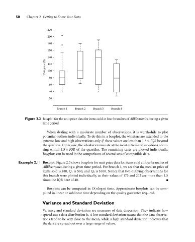
Figure 2.3 Boxplot for the unit price data for items sold at four branches of AllElectronics during a given
time period.

When dealing with a moderate number of observations, it is worthwhile to plot
potential outliers individually. To do this in a boxplot, the whiskers are extended to the
extreme low and high observations only if these values are less than 1.5 × IQR beyond
the quartiles. Otherwise, the whiskers terminate at the most extreme observations occur-
ring within 1.5 × IQR of the quartiles. The remaining cases are plotted individually.
Boxplots can be used in the comparisons of several sets of compatible data.

Example 2.11 Boxplot. Figure 2.3 shows boxplots for unit price data for items sold at four branches of
AllElectronics during a given time period. For branch 1, we see that the median price of
items sold is $80, Q 1 is $60, and Q 3 is $100. Notice that two outlying observations for
this branch were plotted individually, as their values of 175 and 202 are more than 1.5
times the IQR here of 40.

Boxplots can be computed in O(nlogn) time. Approximate boxplots can be com-
puted in linear or sublinear time depending on the quality guarantee required.

Variance and Standard Deviation

Variance and standard deviation are measures of data dispersion. They indicate how
spread out a data distribution is. A low standard deviation means that the data observa-
tions tend to be very close to the mean, while a high standard deviation indicates that
the data are spread out over a large range of values.