Page 90 -

3:15
Page 53
#15
HAN 09-ch02-039-082-9780123814791
2011/6/1
2.2 Basic Statistical Descriptions of Data 53

Table 2.1 A Set of Unit Price Data for Items
Sold at a Branch of AllElectronics
Unit price Count of
($) items sold
40 275
43 300
47 250
− −
74 360
75 515
78 540
− −
115 320
117 270
120 350

120
110 Q 3
Branch 2 (unit price $) 90 Median
100

80
70
60
50 Q 1
40
40 50 60 70 80 90 100 110 120
Branch 1 (unit price $)

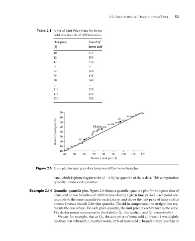
Figure 2.5 A q-q plot for unit price data from two AllElectronics branches.

data, which is plotted against the (i − 0.5)/M quantile of the x data. This computation
typically involves interpolation.

Example 2.14 Quantile–quantile plot. Figure 2.5 shows a quantile–quantile plot for unit price data of
items sold at two branches of AllElectronics during a given time period. Each point cor-
responds to the same quantile for each data set and shows the unit price of items sold at
branch 1 versus branch 2 for that quantile. (To aid in comparison, the straight line rep-
resents the case where, for each given quantile, the unit price at each branch is the same.
The darker points correspond to the data for Q 1 , the median, and Q 3 , respectively.)
We see, for example, that at Q 1 , the unit price of items sold at branch 1 was slightly
less than that at branch 2. In other words, 25% of items sold at branch 1 were less than or