Page 487 - Design and Operation of Heat Exchangers and their Networks

470 Appendix

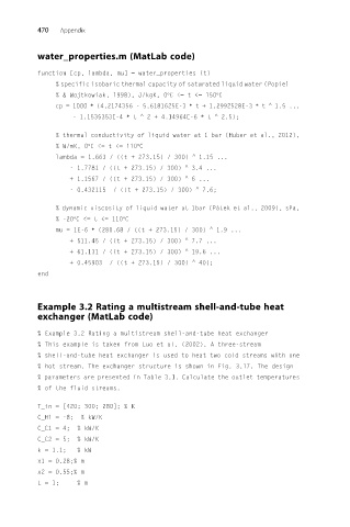
water_properties.m (MatLab code)

function [cp, lambda, mu] = water_properties (t)
% specific isobaric thermal capacity of saturated liquid water (Popiel
% & Wojtkowiak, 1998), J/kgK, 0°C <= t <= 150°C
cp = 1000 ∗ (4.2174356 - 5.6181625E-3 ∗ t + 1.2992528E-3 ∗ t ^ 1.5 ...
- 1.1535353E-4 ∗ t ^ 2 + 4.14964E-6 ∗ t ^ 2.5);
% thermal conductivity of liquid water at 1 bar (Huber et al., 2012),
% W/mK, 0°C <= t <= 110°C
lambda = 1.663 / ((t + 273.15) / 300) ^ 1.15 ...
- 1.7781 / ((t + 273.15) / 300) ^ 3.4 ...
+ 1.1567 / ((t + 273.15) / 300) ^ 6 ...
- 0.432115 / ((t + 273.15) / 300) ^ 7.6;

% dynamic viscosity of liquid water at 1bar (Pátek et al., 2009), sPa,
% -20°C <= t <= 110°C
mu = 1E-6 ∗ (280.68 / ((t + 273.15) / 300) ^ 1.9 ...
+ 511.45 / ((t + 273.15) / 300) ^ 7.7 ...
+ 61.131 / ((t + 273.15) / 300) ^ 19.6 ...
+ 0.45903 / ((t + 273.15) / 300) ^ 40);
end

Example 3.2 Rating a multistream shell-and-tube heat
exchanger (MatLab code)

% Example 3.2 Rating a multistream shell-and-tube heat exchanger
% This example is taken from Luo et al. (2002). A three-stream
% shell-and-tube heat exchanger is used to heat two cold streams with one
% hot stream. The exchanger structure is shown in Fig. 3.17. The design
% parameters are presented in Table 3.1. Calculate the outlet temperatures
% of the fluid streams.

T_in = [420; 300; 280]; % K
C_H1 = -8; % kW/K
C_C1 = 4; % kW/K
C_C2 = 5; % kW/K
k = 1.1; % kW
x1 = 0.28;% m
x2 = 0.55;% m
L= 1; % m