Page 77 - Design and Operation of Heat Exchangers and their Networks

64 Design and operation of heat exchangers and their networks

exchanger are constant; there is no phase change in the heat exchanger;
and the disturbances in thermal flow rates, heat transfer coefficients, and
inlet fluid temperatures are small. Then, the nonlinear terms in the mathe-
matical model for dynamic thermal analysis of heat exchangers can be
linearized.
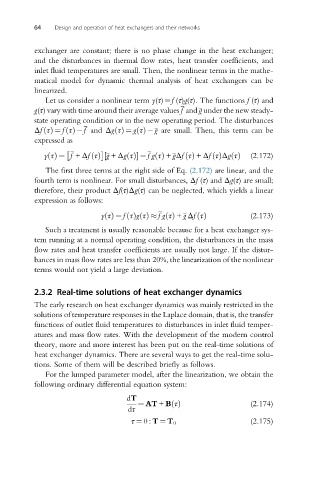
Let us consider a nonlinear term y(τ)¼f (τ)g(τ). The functions f (τ) and
g(τ) vary with time around their average values f and g under the new steady-
state operating condition or in the new operating period. The disturbances
Δf τðÞ ¼ f τðÞ f and Δg τðÞ ¼ g τðÞ g are small. Then, this term can be
expressed as

y τðÞ ¼ f + Δf τðÞ g + Δg τðÞ½ Š ¼ fg τðÞ + gΔf τðÞ + Δf τðÞΔg τðÞ (2.172)
The first three terms at the right side of Eq. (2.172) are linear, and the
fourth term is nonlinear. For small disturbances, Δf (τ) and Δg(τ) are small;
therefore, their product Δf(τ)Δg(τ) can be neglected, which yields a linear
expression as follows:

y τðÞ ¼ f τðÞg τðÞ fg τðÞ + g Δf τðÞ (2.173)
Such a treatment is usually reasonable because for a heat exchanger sys-
tem running at a normal operating condition, the disturbances in the mass
flow rates and heat transfer coefficients are usually not large. If the distur-
bances in mass flow rates are less than 20%, the linearization of the nonlinear
terms would not yield a large deviation.

2.3.2 Real-time solutions of heat exchanger dynamics

The early research on heat exchanger dynamics was mainly restricted in the
solutions of temperature responses in the Laplace domain, that is, the transfer
functions of outlet fluid temperatures to disturbances in inlet fluid temper-
atures and mass flow rates. With the development of the modern control
theory, more and more interest has been put on the real-time solutions of
heat exchanger dynamics. There are several ways to get the real-time solu-
tions. Some of them will be described briefly as follows.
For the lumped parameter model, after the linearization, we obtain the
following ordinary differential equation system:

dT
¼ AT + B τðÞ (2.174)
dτ
τ ¼ 0 : T ¼ T 0 (2.175)