Page 56 - Determinants and Their Applications in Mathematical Physics

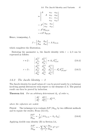
3.6 The Jacobi Identity and Variants 41
A a 21 a 23

Aa 31
a 33
=
a 11
a 13

a 41 a 43

a 11
= A 2 a 13
a 41 a 43

2
= A M 23,24
2
= σA A 23,24 .
Hence, transposing J,

A 22
J = A 24 = AA 23,24
A 32 A 34

which completes the illustration.
Restoring the parameter n, the Jacobi identity with r =2, 3 can be
expressed as follows:
(n)
A A (n) (n)

r =2: ip iq = A n A . (3.6.4)
(n)
(n)
A A ij,pq
jp jq
(n) (n) (n)
A A A
ip iq ir
(n) (n) (n) 2 (n)
r =3: A A A = A A . (3.6.5)

n ijk,pqr
jp jq jr
(n) (n)
A A A
(n)
kp kq kr
3.6.2 The Jacobi Identity — 2
The Jacobi identity for small values of r can be proved neatly by a technique
involving partial derivatives with respect to the elements of A. The general
result can then be proved by induction.
Theorem 3.4. For an arbitrary determinant A n of order n,

A ij A iq
n ip,jq
n = A ,
A pj A pq n
n n
where the cofactors are scaled.
Proof. The technique is to evaluate ∂A /∂a pq by two different methods
ij
and to equate the results. From (3.2.15),
∂A ij 1
= AA ip,jq − A ij A pq . (3.6.6)
A 2
∂a pq
Applying double-sum identity (B) in Section 3.4,
∂A ij ∂a rs
is
= − A A rj
∂a pq
r s ∂a pq