Page 223 - Digital Analysis of Remotely Sensed Imagery

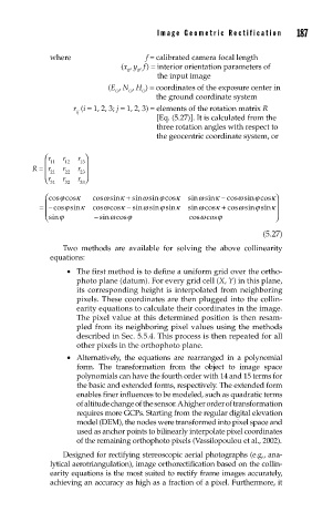
Image Geometric Rectification 187

where f = calibrated camera focal length
(x , y , f ) = interior orientation parameters of
0 0
the input image
(E , N , H ) = coordinates of the exposure center in
O O O
the ground coordinate system
r (i = 1, 2, 3; j = 1, 2, 3) = elements of the rotation matrix R
ij
[Eq. (5.27)]. It is calculated from the
three rotation angles with respect to
the geocentric coordinate system, or

r ⎛ r r ⎞
R = ⎜ r 11 r 12 r 13 ⎟
⎜ 21 22 23 ⎟
r r ⎠
32 33
r ⎝ 31
ω
ω
⎛ cos coosκ cos sinκ + sin sin cosκ sin sinκ − cos sin coosκ⎞
ω
ω
ϕ
ϕ
ϕ
= − ⎜ cos sinκ cos cosκ − sin sin sinκ sin cosκ + ccos sin sinω ϕ κ⎟
ϕ
ω
ω
ω
ϕ
⎜ ⎝ sinϕ − sin cosϕ cos cosϕ ⎟ ⎠
ω
ω

(5.27)
Two methods are available for solving the above collinearity
equations:
• The first method is to define a uniform grid over the ortho-
photo plane (datum). For every grid cell (X, Y) in this plane,
its corresponding height is interpolated from neighboring
pixels. These coordinates are then plugged into the collin-
earity equations to calculate their coordinates in the image.
The pixel value at this determined position is then resam-
pled from its neighboring pixel values using the methods
described in Sec. 5.5.4. This process is then repeated for all
other pixels in the orthophoto plane.
• Alternatively, the equations are rearranged in a polynomial
form. The transformation from the object to image space
polynomials can have the fourth order with 14 and 15 terms for
the basic and extended forms, respectively. The extended form
enables finer influences to be modeled, such as quadratic terms
of altitude change of the sensor. A higher order of transformation
requires more GCPs. Starting from the regular digital elevation
model (DEM), the nodes were transformed into pixel space and
used as anchor points to bilinearly interpolate pixel coordinates
of the remaining orthophoto pixels (Vassilopoulou et al., 2002).
Designed for rectifying stereoscopic aerial photographs (e.g., ana-
lytical aerotriangulation), image orthorectification based on the collin-
earity equations is the most suited to rectify frame images accurately,
achieving an accuracy as high as a fraction of a pixel. Furthermore, it