Page 108 - Dynamic Vision for Perception and Control of Motion

3 Subjects and Subject Classes
92

2.5 m would have the local (say, the front) wheels leave the ground. Since, in gen-
eral, there will be forces on the rear wheels, pitch acceleration downward will also
result. These are conditions well-known from rallye-driving. Vertical curvatures
can be recognized by vision in the look-ahead range so that these dynamic effects
on vehicle motion can be foreseen and will not come by surprise.
Autonomous vehicles going cross-country have to be aware of these conditions
to select proper speed as well as the shape and location of the track for steering.
This is a complex optimization task: On the tracks, for the wheels on both sides of
the vehicle the vertical surface profiles have to be recognized at least approxi-
mately correctly. From this information, the vertical and rotational perturbations
(heave, pitch, and roll) to be expected can be estimated. Since lateral control leaves
a degree of freedom in the curvature of the horizontal track through steering, a
compromise allowing a safe trajectory at a good speed with acceptable perturba-
tions from uneven terrain has to be found. This will remain a challenging task for
some time to come.
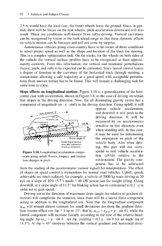
Slope effects on longitudinal motion: Figure 3.18 is a generalization of the hori-
zontal case with acceleration, shown in Figure 3.8, to the case of driving on terrain
that slopes in the driving direction. Now, the all dominating gravity vector has a
component of magnitude (m · g · sinɛ) in the driving direction. Going uphill, it will
oppose vehicle acceleration,
Axle distance “a” and downhill it will push in the
Center driving direction. It will be
of gravity “cg”
Gravity component + F p measured by an accelerometer
ímg sin ɛ ǻV f ǻș p
ɛ sensitive in this direction even
í F h
ǻV r p cg + ɛ when standing still. In this case,
+ ɛ it may be used for determining
Slope angle ɛ the orientation in pitch of the
+ F mg
p Remaining propulsive vehicle body. Also when driv-
force after subtraction
of gravity component ing, this part will not corre-
spond to real vehicle accelera-
Figure 3.18. Longitudinal acceleration compo-
nents going uphill: Forces, torques, and orienta- tion (dV/dt) relative to the
tion changes in pitch environment. The gravity com-
ponent has to be subtracted
from the reading of the accelerometer (sensor signal) for interpretation. The effect
of slopes on speed control is tremendous for normal road vehicles. Uphill, speeds
achievable are much reduced; for example, a vehicle of 2000 kg mass driving at 20
m/s on a slope of 10% (5.7°) needs § 40 kW power just for weight lifting. Going
downhill, at a slope angle of 11.5° the braking action has to correspond to 0.2 · g in
order not to gain speed.
Driving not in the direction of maximum slope (angle ǻȥ relative to gradient di-
rection) will complicate the situation, since there will be a lateral force component
acting in addition to the longitudinal one. Note that the longitudinal component
a Lon will remain almost constant for small deviations ǻȥ from the gradient direc-
tion (cosine-effect cos ǻȥ § 1 up to 15°, that is, a Lon § a grad = g · sin ɛ), while the
lateral component will increase linearly according to the sine of the relative head-
ing angle ǻȥ (a lat § g · sin ɛ · sin ǻȥ, yielding § 0.2 g · sin ɛ for an angle ǻȥ of
11.5°). At ǻȥ = 45° (midway between the vertical gradient and horizontal direc-