Page 112 - Dynamic Vision for Perception and Control of Motion

3 Subjects and Subject Classes
96

2
2
2
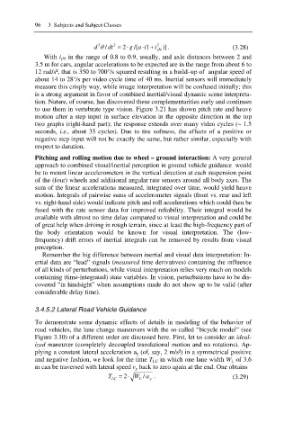
d T / dt ˜ /[a ˜ (1 i )] . (3.28)

2 g
yN
With i yN in the range of 0.8 to 0.9, usually, and axle distances between 2 and
3.5 m for cars, angular accelerations to be expected are in the range from about 6 to
12 rad/s², that is 350 to 700°/s squared resulting in a build–up of angular speed of
about 14 to 28°/s per video cycle time of 40 ms. Inertial sensors will immediately
measure this crisply way, while image interpretation will be confused initially; this
is a strong argument in favor of combined inertial/visual dynamic scene interpreta-
tion. Nature, of course, has discovered these complementarities early and continues
to use them in vertebrate type vision. Figure 3.21 has shown pitch rate and heave
motion after a step input in surface elevation in the opposite direction in the top
two graphs (right-hand part); the response extends over many video cycles (~ 1.5
seconds, i.e., about 35 cycles). Due to tire softness, the effects of a positive or
negative step input will not be exactly the same, but rather similar, especially with
respect to duration.
Pitching and rolling motion due to wheel – ground interaction: A very general
approach to combined visual/inertial perception in ground vehicle guidance would
be to mount linear accelerometers in the vertical direction at each suspension point
of the (four) wheels and additional angular rate sensors around all body axes. The
sum of the linear accelerations measured, integrated over time, would yield heave
motion. Integrals of pairwise sums of accelerometer signals (front vs. rear and left
vs. right-hand side) would indicate pitch and roll accelerations which could then be
fused with the rate sensor data for improved reliability. Their integral would be
available with almost no time delay compared to visual interpretation and could be
of great help when driving in rough terrain, since at least the high-frequency part of
the body orientation would be known for visual interpretation. The (low-
frequency) drift errors of inertial integrals can be removed by results from visual
perception.
Remember the big difference between inertial and visual data interpretation: In-
ertial data are “lead” signals (measured time derivatives) containing the influence
of all kinds of perturbations, while visual interpretation relies very much on models
containing (time-integrated) state variables. In vision, perturbations have to be dis-
covered “in hindsight” when assumptions made do not show up to be valid (after
considerable delay time).

3.4.5.2 Lateral Road Vehicle Guidance

To demonstrate some dynamic effects of details in modeling of the behavior of
road vehicles, the lane change maneuvers with the so-called “bicycle model” (see
Figure 3.10) of a different order are discussed here. First, let us consider an ideal-
ized maneuver (completely decoupled translational motion and no rotations). Ap-
plying a constant lateral acceleration a y (of, say, 2 m/s²) in a symmetrical positive
and negative fashion, we look for the time T LC in which one lane width W L of 3.6
m can be traversed with lateral speed v y back to zero again at the end. One obtains
T ˜ W / a . (3.29)
2
LC L y