Page 114 - Dynamic Vision for Perception and Control of Motion

3 Subjects and Subject Classes
98

as springs in the lateral direction with an approximately linear characteristic for
small angles of attack (|Į| < § 3°); only this regime is considered here. For the test
vehicle VaMoRs, this allows lateral accelerations up to about 0.4 g = 4 m/s² in the
linear range.
With k T as the lateral tire force coefficient linking vertical tire force F N = m WL·g
(wheel load due to gravity) via angle of attack to lateral tire force F y , there follows
F yf k ˜ T f ˜D F Nf ; F yr k ˜ T r ˜D F Nr . (3.30)
If the vehicle weight is distributed almost equally onto all wheels of a four-
wheel vehicle, m WL is close to one quarter of total vehicle mass; in the bicycle
model, it is close to one half the total mass both on the front and rear axle. Defin-
ing the mass related lateral force coefficient k ltf
k ltf F y /(m ˜ WL f ) k ˜D T g (in m/s²/rad) , (3.31)
and multiplying this coefficient with both the actual wheel load (in terms of mass)
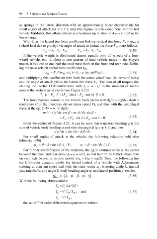
and the angle of attack yields the lateral tire force F y . The sum of all torques (in-
cluding the inertial D’Alembert-term with I z = m · i z² as the moment of inertia
around the vertical axis) yields (see Figure 3.23)

I ˜ F ˜ (F ˜ sin F ˜ cos ) lf 0 . (3.32)
O
O
\
˜
l
yf
r
yr
z
xf
The force balance normal to the vehicle body yields with dȤ/dt = dȤ/ds · ds/dt =
(curvature C of the trajectory driven times speed V), and thus with the centrifugal
force at the cg: C ·V² = m· V· dȤ/dt
˜
mV dF / dt ˜ cosE m d / dt ˜ sin E
˜˜

F F ˜ sin O F ˜ cos O 0. (3.33)
yr xf yf
From the center of Figure 3.23, it can be seen that trajectory heading Ȥ is the
sum of vehicle body heading ȥ and side slip angle ȕ (Ȥ = ȥ + ȕ) and thus
d /dt F d \ / dt dE / dt. (3.34)
For small angles of attack at the wheels, the following relations hold after
[Mitschke 1990]:
˜
˜
D E O d \ / dt l / ; D E d \ / dt l /V .
V
f f r r (3.35)
For further simplification of the relations, the cg is assumed to lie at the center
between the front and rear axles (l f = l r = a/2), so that half of the vehicle mass rests
on each axle (wheel of bicycle model: F Nr = F Nf = mg/2). Then, the following lin-
ear fifth-order dynamic model for lateral control of a vehicle with Ackermann-
steering at constant speed and with the state vector x La (steering angle Ȝ, inertial
yaw rate dȥ/dt, slip angle ȕ, body heading angle ȥ, and lateral position y) results:
T
O\

\
E
x [ , , , , ] . (3.36)
y
La
With the following abbreviations:
2
2
i [/( /2)] ;
i
a
zB
z
2
T ˜ zB /k ltf ; and (3.37)
V i
\
T V /k ltf ,
E
the set of first-order differential equations is written