Page 116 - Dynamic Vision for Perception and Control of Motion

3 Subjects and Subject Classes
100

The eigenfrequency of human
A’ 2 O max,2 = A’ 2 · IJ 2 Idealized “doublet” for arms and legs is in the 2 Hz range (Ȧ
IJĺ 0 such that the -1
product A’ i · IJ i ²remains = 12.6 s ) so that the first-order de-
constant (O max,i · IJ i ) lay effects at lower speeds will
O max,1 = A’ 1 · IJ 1
hardly be noticeable by humans too.
Steering angle O (state)
IJ O max = A · IJ
A’ 1 However, when speed increases,
0 there will be strong dynamical ef-
A 2 · IJ 0 time
0 fects. This will be shown with an
íA 0
IJ T doublet = 2 · IJ idealized maneuver: The doublet as
IJ 1 0 0
shown in Figure 3.12 is redrawn in
t + IJ 0 t + 2IJ 0
íA’ 1
Figure 3.25 on an absolute timescale
with control output beginning at zero.
From Table 3.2, it can be seen that
IJ 2
Steering rate dO/dt time T 2, in which a preset accelera-
í A’ 2 piecewise constant control input (doublet) tion limit can be reached with con-
stant control output A, decreases rap-
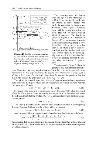
Figure 3.25. Doublet in constant steer rate
idly with speed V. Let us, therefore,
u ff (·) = dO/dt as control time history over
look at the limiting case for the dou-
two periods IJ with opposite sign of ampli-
blet when its duration 2IJ goes to
tude ± A’ yields an “ideal impulse” in steer
zero.
angle for heading change and IJĺ 0
The doublets in Figure 3.25 can be
generated as a sum of three step func-
tions. From 0 to IJ the only step function u 1(t) = A’·1(t) is active; from IJ to 2IJ a su-
perposition of two step functions, the second one delayed by IJ, yields u 2(t) =
A’·[1(t) – 2·1(t – IJ)]. For the third phase from 2IJ forward, the previous function
plus a step delayed by 2IJ is valid: u(t) = u 2(t) + A’· 1(t – 2IJ).
This yields the control input time history of superimposed delayed step func-
tions shown in the figure, which can be summarized as control function with the
two parameters A’ and IJ:
W
˜
t
( )
ut A ' [1( ) 2(t ) 1(t 2 )] . (3.40)

W
For making the transition to distribution theory [Papoulis 1962] when the period
of the doublet IJ goes to zero, we rewrite the amplitude A’ in Equation 3.40 under
the side constraint that the product (A i’· IJ i²) is kept constant when duration IJ i is de-
creased to zero
2
'( , )W
At A / W . (3.41)
i i i
This (purely theoretical) time function has a simple description in the frequency
domain; Equation 3.40 can now be written with A = constant
2
(, )
ut W A˜ [1( ) 2 1(t W ) 1(t ˜ W )]/ W 2 . (3.42)
t
˜

As a two-step difference approximation based on step functions, there follows
t
W
1( ) 1(t W ) 1(t ) 1(t 2 ) º ˜ W
ª
ut A˜ W . (3.43)
(, ) W
« »
¬ W W ¼
Recognizing that each expression in the square bracket describes a Dirac impulse
for IJ toward 0, nice theoretical results for the (ideal) doublet and doublet responses
are obtained easily.