Page 118 - Dynamic Vision for Perception and Control of Motion

3 Subjects and Subject Classes
102

ble. These differences in dynamic behavior have to be taken into account when
computing expectations after a control input in steering angle. They play an impor-
tant role in decision-making, for example, when the amplitude of a control input as
a function of speed driven has to be determined as one of the situational aspects.

Lane changes with realistic control input: The idealized relations discussed
above yield a good survey of the basic behavioral properties of road vehicles as a
function of speed driven. Real maneuvers have to take the saturation effects in
steering rate into account. Analytical solutions become rather complex for these
conditions. Simulation results with the nonlinear set of equations are easily avail-
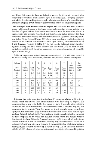
able today. Table 3.4 and Figure 3.27 show some simulation results for a typical
vehicle. Three different characteristic control input times T C have been selected: 6,
4, and 2 seconds (column 1, Table 3.4) for two speeds. Column 2 shows the steer-
ing rates leading to a final lateral offset of one lane width (3.75 m) after the tran-
sients have settled, with the other parameters pre–selected (duration of central 0-
input time beside T C ).
Table 3.4. Expectations for lane change maneuvers ('y = 3.75 m) with preset control in-
put times according to the 5th-order bicycle model with piecewise constant steering rates

Column 1 2 3 4 5 6 7 8 Re-
state mark:
T C
Speed control dȜ/dt Ȝ max ȥ max ȕ max a ymax v ymax transit. Figure
V/km/h time /s / °/s / ° / ° / ° / m/s 2 / m/s time /s 3.27
40 6 0.9 1.4 6.4 0.16 0.7 1.2 6.5
40 4 3.1 3.1 9.6 0.36 1.5 1.8 4.5
40 2 24 12 18.5 1.7 5.2 3.2 2.7
100 6 0.16 0.22 2.5 0.5 0.6 1.2 7.9 (a)
100 4 0.5 0.5 3.7 0.95 1.1 1.6 6.0
100 2 3.9 2 6.5 2.6 2.7 2.35 4.4 (b)
100 6 0.18 0.23 2.2 0.5 0.6 1 7.9
100 4 0.64 0.51 3.2 0.9 1 1 1.45 6
100 2 5.1 2 6 2.2 2.3 2.26 4.4 (c)

It is seen that state transition time (column 8) increases relative to T C with in-
creased speed; the ratio of these times increases with decreasing T C. Figure 3.27a
(corresponding to row 4 in Table 3.4, maneuver time 6 seconds) shows that the
state transitions are almost finished when the control input is finished. Figure 3.27b
(corresponding to row 6 in Table 3.4, maneuver time 2 seconds) shows in the lower
right part, that maximum (negative) lateral acceleration occurs after control input
has been finished (is back to 0). The maximum positive acceleration has increased
4.5-fold compared to a), while the maximal lateral speed has almost doubled.
Steering rate (column 2) for the 2-second maneuver is 24 times as high as for the 6-
second maneuver while the maximum steering angle increased by a factor of 9
(column 3). Maximum slip angle (column 5) increases fivefold while the maximum
heading angles (column 4) differ by a factor of only 2.6. In the short maneuver
with T C = 2 [1/3 of case a)], state transition needs about twice the control input time