Page 163 - Dynamics of Mechanical Systems

0593_C05_fm Page 144 Monday, May 6, 2002 2:15 PM

144 Dynamics of Mechanical Systems

N
O X
X
n 11
n
N Y 21
G 1
θ 1
O 2
n
B 1 G 2 13
θ 2 n
O 3 23
G 3 n
N1
B 2 O 4
θ 3
B O N-1
3
θ G N-1 n N3
N N-1 O N
Z
B N-1 G N
θ N
Z B N
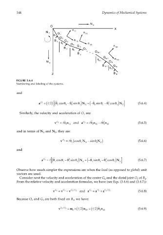
FIGURE 5.6.4
Numbering and labeling of the systems.
and
˙˙
˙˙
a G1 = (l 2) θ 1 ( [ cosθ 1 − θ 2 ˙ 1 sinθ 1) N +− ( θ 1 sinθ 1 − θ 2 ˙ 1 cosθ 1) N Z] (5.6.4)
X
Similarly, the velocity and acceleration of O are:
2
˙˙
n − lθ
v O 2 = lθ ˙ 1 11 a O 2 = lθ 1 11 2 ˙ 1 n 13 (5.6.5)
n and
and in terms of N and N , they are:
Z
X
v O 2 = lθ ˙ 1 (cosθ 1 N − sinθ 1 N ) (5.6.6)
X
Z
and

˙˙
˙˙
a O 2 = l θ 1 ( [ cosθ 1 − θ 2 ˙ 1 sinθ 1) N +− ( θ 1 sinθ 1 − θ 2 ˙ 1 cosθ 1) N Z] (5.6.7)
X
Observe how much simpler the expressions are when the local (as opposed to global) unit
vectors are used.
Consider next the velocity and acceleration of the center G and the distal joint O of B .
2
3
2
From the relative velocity and acceleration formulas, we have (see Eqs. (3.4.6) and (3.4.7)):
2 /
2 /
v G 2 = v O 2 + v GO 2 and a G 2 = a O 2 + a GO 2 (5.6.8)
Because O and G are both fixed on B , we have:
2
2
2
×
2 /
v GO 2 = ωω 2 (l 2) n = (l 2)θ ˙ 2 n 21 (5.6.9)
23