Page 448 - Dynamics of Mechanical Systems

0593_C12_fm Page 429 Monday, May 6, 2002 3:11 PM

Generalized Dynamics: Kane’s Equations and Lagrange’s Equations 429

By substituting from Eqs. (12.3.15), (12.3.17), (12.3.18), (12.3.19), and (12.3.20), the govern-
ing equations become:

mx ˙˙ − m(l + x )θ ˙ 2 = mgcos + kx − 2 kx (12.3.32)
θ
1 1 2 1
m 2 + )θ
θ
mx ˙˙ − ( l x ˙ 2 = mgcos + kx + kx (12.3.33)
2 2 3 1
θ
m 3 + )θ
mx ˙˙ − ( l x ˙ 2 = mgcos − 2 kx + kx (12.3.34)
3 3 3 2
and
[
]
m l + ( x ) +(2 l + x ) +(3 l + x ) θ +( ) 3 ML θ
2
2
2
2 ˙˙
˙˙
1
1
2
3
m l + ( [ x x ) ]
˙
˙
+ 2 x x ) θ ˙ +(2 l + x x ) θ ˙ +(3 l + ˙ θ ˙ (12.3.35)
1 1 2 2 3 3
=− Mg L ( ) 2 sinθ − mg l + x + x + )sinθ
(6
x
3
1
2
Equations (12.3.22), (12.3.23), (12.3.24), and (12.3.25) are seen to be identical to Eqs.
(12.2.32), (12.2.33), (12.2.34), and (12.2.35) obtained using Kane’s equations.
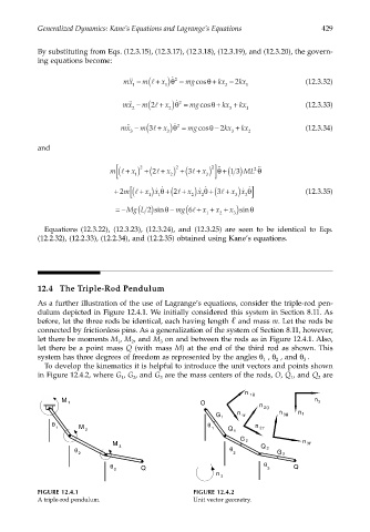
12.4 The Triple-Rod Pendulum
As a further illustration of the use of Lagrange’s equations, consider the triple-rod pen-
dulum depicted in Figure 12.4.1. We initially considered this system in Section 8.11. As
before, let the three rods be identical, each having length and mass m. Let the rods be
connected by frictionless pins. As a generalization of the system of Section 8.11, however,
let there be moments M , M , and M on and between the rods as in Figure 12.4.1. Also,
1 2 3
let there be a point mass Q (with mass M) at the end of the third rod as shown. This
system has three degrees of freedom as represented by the angles θ , θ , and θ .
1 2 3
To develop the kinematics it is helpful to introduce the unit vectors and points shown
in Figure 12.4.2, where G , G , and G are the mass centers of the rods, O, Q , and Q are
1 2 3 1 2
n 1 θ
M 1 O n 2
n 2 θ
n n 3 θ n 1
G 1 1 r
θ θ
1 M 2 1 Q 1 n 2 r
G 2
M n 3 r
θ 3 θ Q 2
2 2 G 3
θ θ
3 Q 3 Q
n
3
FIGURE 12.4.1 FIGURE 12.4.2
A triple-rod pendulum. Unit vector geometry.