Page 452 - Dynamics of Mechanical Systems

0593_C12_fm Page 433 Monday, May 6, 2002 3:11 PM

Generalized Dynamics: Kane’s Equations and Lagrange’s Equations 433

to Eqs. (8.11.1), (8.11.2), and (8.11.3) reportedly developed using d’Alembert’s principle.
Although the details of that development were not presented, the use of Lagrange’s
equations has the clear advantage of providing the simpler analysis. As noted before, the
simplicity and efficiency of the Lagrangian analysis stem from the avoidance of the
evaluation of accelerations and from the automatic elimination of nonworking constraint
forces. In the following section, we outline the extension of this example to include N rods.

12.5 The N-Rod Pendulum
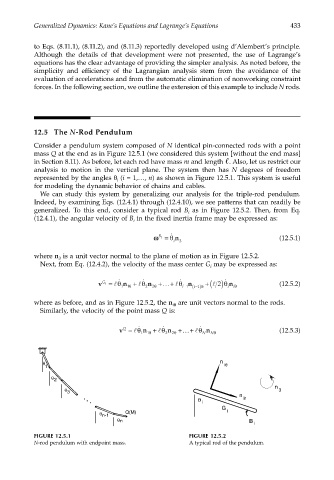
Consider a pendulum system composed of N identical pin-connected rods with a point
mass Q at the end as in Figure 12.5.1 (we considered this system [without the end mass]
in Section 8.11). As before, let each rod have mass m and length . Also, let us restrict our
analysis to motion in the vertical plane. The system then has N degrees of freedom
represented by the angles θ (i = 1,…, n) as shown in Figure 12.5.1. This system is useful
i
for modeling the dynamic behavior of chains and cables.
We can study this system by generalizing our analysis for the triple-rod pendulum.
Indeed, by examining Eqs. (12.4.1) through (12.4.10), we see patterns that can readily be
generalized. To this end, consider a typical rod B as in Figure 12.5.2. Then, from Eq.
i
(12.4.1), the angular velocity of B in the fixed inertia frame may be expressed as:
i
˙
ωω = θ n (12.5.1)
B 1
i 3
where n is a unit vector normal to the plane of motion as in Figure 12.5.2.
3
Next, from Eq. (12.4.2), the velocity of the mass center G may be expressed as:
i
n + lθ
v = lθ ˙ 11 θ ˙ 2 n +…+ lθ ˙ i−1 n i− ( 1 )θ +(l 2 ˙ i )θ n iθ (12.5.2)
G i
θ
2
where as before, and as in Figure 12.5.2, the n are unit vectors normal to the rods.
iθ
Similarly, the velocity of the point mass Q is:
n + lθ
v = lθ ˙ 11 θ ˙ 2 n +…+ lθ ˙ N n Nθ (12.5.3)
Q
θ
2

θ n iθ
1
θ
2
n
θ 3 3
n
θ i ir
G
θ n-1 Q(M) i
θ n B i

FIGURE 12.5.1 FIGURE 12.5.2
N-rod pendulum with endpoint mass. A typical rod of the pendulum.