Page 535 - Dynamics of Mechanical Systems

0593_C15_fm Page 516 Tuesday, May 7, 2002 7:05 AM

516 Dynamics of Mechanical Systems

P (m) Q (m)
1
2
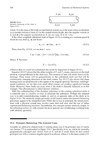
FIGURE 15.3.3
Dynamic balancing of the shaft of Q (m) P (m)
Figure 15.3.2. 1 2
ˆ
where M is the mass of the body (or mechanical system), a is the mass center acceleration
G
in an inertial reference frame R, I is the central inertia dyadic, ωω ωω is the angular velocity in
ˆ
R, and αα αα is the angular acceleration in R. (In our case, M is M + 2m.)
If the offset weighted cylindrical shaft of Figure 13.3.2 is rotating at a uniform speed Ω
about its axis, then a , ωω ωω, and αα αα are:
G
=
a = 0, ωω Ω n , αα = 0 (15.3.5)
G 1
Then, from Eq. (15.3.2), we see that I · ω is:

) ]
[
I⋅ωω = I⋅Ω n = mr 2 +(M 2 r 2 Ω n + 2mrl Ω n (15.3.6)
1 1 2
*
Hence, T becomes:
T =−2mrlΩ 2 n (15.3.7)
*
3
(Observe that we could have predicted this result by inspection of Figure 15.3.2.)
Equation (15.3.7) shows that the offset weights of P and P create a moment on the shaft
2
1
about n or perpendicular to the shaft axis. This moment in turn will create forces on the
3
bearings. These forces will be perpendicular to the cylindrical shaft axis but will be
continuously changing directions as the shaft rotates. Eq. (15.3.7) also shows that these
bearing forces are proportional to the square of the angular speed Ω. Therefore, with high-
speed machinery, we see that even small offset masses can produce significant bearing
loads. Moreover, these loads can occur even if the shaft is statically balanced as in this
example. This phenomenon is called dynamic unbalance.
With this understanding of the dynamic unbalance of the rotating cylindrical shaft, it
is relatively easy to conceive of ways to eliminate the unbalance. Perhaps the simplest
way is to add counterbalancing weights Q and Q at opposite sides of the shaft, as in
1
2
Figure 15.3.3. The relatively simple geometry of this system makes the dynamic balancing
procedure appear to be straightforward. While this is true in principal, the actual proce-
dure with a physical system may involve some trial and error and the use of rather
sophisticated balancing machines. Nevertheless, the concepts remain relatively simple. In
the following section, we will consider the more general case of balancing a rotating body
with arbitrary geometry.

15.4 Dynamic Balancing: The General Case
Consider an arbitrarily shaped body B rotating about one of its principal axes of inertia
(see Section 7.7) as represented in Figure 15.4.1. Specifically, let n , n , and n be mutually
2
1
3
perpendicular principal unit vectors fixed in B, and let B rotate about its first central
principal axis with a constant angular speed Ω as shown, where G is the mass center of B.