Page 59 - Earth's Climate Past and Future

CHAPTER 2 • Climate Archives, Data, and Models 35

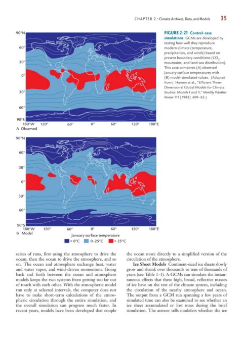
90°N FIGURE 2-21 Control-case
simulations GCMs are developed by
testing how well they reproduce
60° modern climate (temperature,
precipitation, and winds) based on
present boundary conditions (CO ,
2
30° mountains, and land-sea distribution).
This case compares (A) observed
January surface temperatures with
0°
(B) model-simulated values. (Adapted
from J. Hansen et al., “Efficient Three-
Dimensional Global Models for Climate
30° Studies: Models I and II,” Monthly Weather
Review 111 [1983]: 609–62.)

60°

90°S
180°W 120° 60° 0° 60° 120° 180°E
A Observed

90°N

60°

30°

0°

30°

60°

90°S
180°W 120° 60° 0° 60° 120° 180°E
B Model
January surface temperature
< 0°C 0–25°C > 25°C

series of runs, first using the atmosphere to drive the the ocean more directly to a simplified version of the
ocean, then the ocean to drive the atmosphere, and so circulation of the atmosphere.
on. The ocean and atmosphere exchange heat, water Ice Sheet Models Continent-sized ice sheets slowly
and water vapor, and wind-driven momentum. Going grow and shrink over thousands to tens of thousands of
back and forth between the ocean and atmosphere years (see Table 1–1). A-GCMs can simulate the instan-
models keeps the two systems from getting too far out taneous effects that these high, broad, reflective masses
of touch with each other. With the atmospheric model of ice have on the rest of the climate system, including
run only at selected intervals, the computer does not the circulation of the nearby atmosphere and ocean.
have to make short-term calculations of the atmos- The output from a GCM run spanning a few years of
pheric circulation through the entire simulation, and simulated time can also be examined to see whether an
the overall simulation can progress much faster. In ice sheet accumulated or lost mass during the brief
recent years, models have been developed that couple simulation. The answer tells modelers whether the ice