Page 58 - Earth's Climate Past and Future

34 PART I • Framework of Climate Science

components in models are often so crude that they
Last 5 years make the resulting climate simulations less realistic than
those obtained from models that had simply held those
Simulated climate value Spin-up phase of model run climate output data refined representations do the newly added components
components fixed at modern values. Only with more
Model atmosphere
stabilized
perform in a realistic way and make the resulting simu-
lations clearly superior to the earlier versions.
Values used for
Ocean GCMs Models of ocean circulation are at a
slightly more primitive stage of development than atmos-
pheric GCMs. One reason is that climate researchers
know much less about the modern circulation of the
Model atmosphere at rest
oceans, especially critical processes such as the brief but
0 5 10 15 20 intense episodes of deep-water formation at high lati-
Years of elapsed model time
tudes. As a result, scientists do not have as well defined a
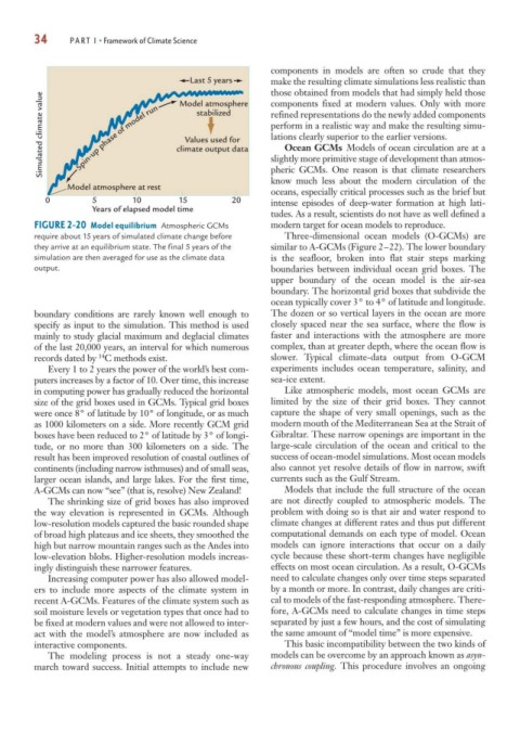
FIGURE 2-20 Model equilibrium Atmospheric GCMs modern target for ocean models to reproduce.
require about 15 years of simulated climate change before Three-dimensional ocean models (O-GCMs) are
they arrive at an equilibrium state. The final 5 years of the similar to A-GCMs (Figure 2–22). The lower boundary
simulation are then averaged for use as the climate data is the seafloor, broken into flat stair steps marking
output. boundaries between individual ocean grid boxes. The
upper boundary of the ocean model is the air-sea
boundary. The horizontal grid boxes that subdivide the
ocean typically cover 3° to 4° of latitude and longitude.
boundary conditions are rarely known well enough to The dozen or so vertical layers in the ocean are more
specify as input to the simulation. This method is used closely spaced near the sea surface, where the flow is
mainly to study glacial maximum and deglacial climates faster and interactions with the atmosphere are more
of the last 20,000 years, an interval for which numerous complex, than at greater depth, where the ocean flow is
14
records dated by C methods exist. slower. Typical climate-data output from O-GCM
Every 1 to 2 years the power of the world’s best com- experiments includes ocean temperature, salinity, and
puters increases by a factor of 10. Over time, this increase sea-ice extent.
in computing power has gradually reduced the horizontal Like atmospheric models, most ocean GCMs are
size of the grid boxes used in GCMs. Typical grid boxes limited by the size of their grid boxes. They cannot
were once 8° of latitude by 10° of longitude, or as much capture the shape of very small openings, such as the
as 1000 kilometers on a side. More recently GCM grid modern mouth of the Mediterranean Sea at the Strait of
boxes have been reduced to 2° of latitude by 3° of longi- Gibraltar. These narrow openings are important in the
tude, or no more than 300 kilometers on a side. The large-scale circulation of the ocean and critical to the
result has been improved resolution of coastal outlines of success of ocean-model simulations. Most ocean models
continents (including narrow isthmuses) and of small seas, also cannot yet resolve details of flow in narrow, swift
larger ocean islands, and large lakes. For the first time, currents such as the Gulf Stream.
A-GCMs can now “see” (that is, resolve) New Zealand! Models that include the full structure of the ocean
The shrinking size of grid boxes has also improved are not directly coupled to atmospheric models. The
the way elevation is represented in GCMs. Although problem with doing so is that air and water respond to
low-resolution models captured the basic rounded shape climate changes at different rates and thus put different
of broad high plateaus and ice sheets, they smoothed the computational demands on each type of model. Ocean
high but narrow mountain ranges such as the Andes into models can ignore interactions that occur on a daily
low-elevation blobs. Higher-resolution models increas- cycle because these short-term changes have negligible
ingly distinguish these narrower features. effects on most ocean circulation. As a result, O-GCMs
Increasing computer power has also allowed model- need to calculate changes only over time steps separated
ers to include more aspects of the climate system in by a month or more. In contrast, daily changes are criti-
recent A-GCMs. Features of the climate system such as cal to models of the fast-responding atmosphere. There-
soil moisture levels or vegetation types that once had to fore, A-GCMs need to calculate changes in time steps
be fixed at modern values and were not allowed to inter- separated by just a few hours, and the cost of simulating
act with the model’s atmosphere are now included as the same amount of “model time” is more expensive.
interactive components. This basic incompatibility between the two kinds of
The modeling process is not a steady one-way models can be overcome by an approach known as asyn-
march toward success. Initial attempts to include new chronous coupling. This procedure involves an ongoing