Page 338 - Electrical Properties of Materials

320 Lasers

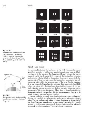
Fig. 12.20
Experimentally measured transverse
mode patterns in a He–Ne laser
having a resonator of rectangular
symmetry (H. Kogelnik and T. Li,
Proc. IEEE 54, pp. 1312–1329, Oct.
1966).

12.8.2 Axial modes

As mentioned in Section 12.5 and shown in Fig. 12.21, laser oscillations are
possible at a number of axial modes, each having an integral number of half-
Resonator loss wavelengths in the resonator. The frequency difference between the nearest
modes is c m /2L (see Exercise 12.7), where L is the length of the resonator,
Laser
gain and c m is the velocity of light in the medium. How can we have a single fre-
quency output? One way is to reduce the length of the resonator so that only
f
one mode exists within the inversion range of the laser. Another technique
c /2L
m is to use the good offices of another resonator. This is shown in Fig. 12.22,
Laser where a so-called Fabry–Perot etalon, a piece of dielectric slab with two par-
output
tially reflecting mirrors, is inserted into the laser resonator. It turns out that the
resonances of this composite structure follow those of the etalon, that is, the
f frequency spacing is c m /2d, where d is the etalon thickness. Since d L,
single frequency operation becomes possible.
Fig. 12.21
Are we not losing too much power by eliminating that many axial modes?
The inversion curve of a laser and the
No, we lose very little power because the modes are not independent of each
possible axial modes as a function of
other. The best explanation is a kind of optical Darwinism or the survival of
frequency.
the fittest. Imagine a pack of young animals (modes) competing for a certain
amount of food (inverted population). If the growth of some of the animals is
prevented, the others grow fatter. This is called mode competition.