Page 281 - Elements of Distribution Theory

P1: JZP
052184472Xc09 CUNY148/Severini June 2, 2005 12:8

9.3 Asymptotic Expansions 267

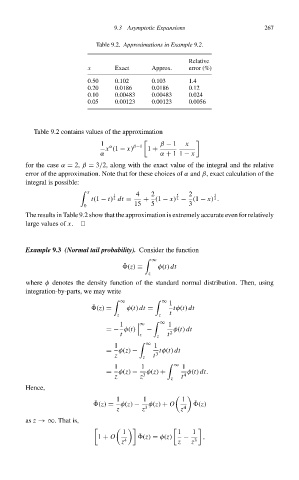
Table 9.2. Approximations in Example 9.2.

Relative
x Exact Approx. error (%)

0.50 0.102 0.103 1.4
0.20 0.0186 0.0186 0.12
0.10 0.00483 0.00483 0.024
0.05 0.00123 0.00123 0.0056

Table 9.2 contains values of the approximation
1 β−1 β − 1 x
α
x (1 − x) 1 +
α α + 1 1 − x
for the case α = 2, β = 3/2, along with the exact value of the integral and the relative
error of the approximation. Note that for these choices of α and β,exact calculation of the
integral is possible:
x
1 4 2 5 2 3
t(1 − t) 2 dt = + (1 − x) 2 − (1 − x) 2 .
0 15 5 3
The results in Table 9.2 show that the approximation is extremely accurate even for relatively
large values of x.

Example 9.3 (Normal tail probability). Consider the function
∞

¯
(z) ≡ φ(t) dt
z
where φ denotes the density function of the standard normal distribution. Then, using
integration-by-parts, we may write
∞ ∞ 1

¯
(z) = φ(t) dt = tφ(t) dt
z z t
1 ∞ ∞ 1

− φ(t) dt
t z z t
=− φ(t) 2
1 ∞ 1
= φ(z) − tφ(t) dt
z z t 3
1 1 ∞ 1
= φ(z) − φ(z) + φ(t) dt.
z z 3 z t 4
Hence,

1 1 1
¯ ¯
(z) = φ(z) − φ(z) + O (z)
z z 3 z 4
as z →∞. That is,

1 1 1
¯
1 + O (z) = φ(z) − ,
z 4 z z 3