Page 280 - Elements of Distribution Theory

P1: JZP
052184472Xc09 CUNY148/Severini June 2, 2005 12:8

266 Approximation of Integrals

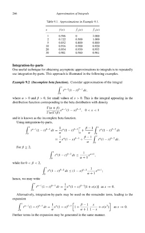
Table 9.1. Approximations in Example 9.1.

x f (x) ˆ f (x) ˆ f (x)
3
2
1 0.596 0 2.000
2 0.722 0.500 1.000
5 0.852 0.800 0.880
10 0.916 0.900 0.920
20 0.954 0.950 0.955
30 0.981 0.980 0.981

Integration-by-parts
One useful technique for obtaining asymptotic approximations to integrals is to repeatedly
use integration-by-parts. This approach is illustrated in the following examples.

Example 9.2 (Incomplete beta function). Consider approximation of the integral
x

t α−1 (1 − t) β−1 dt,
0
where α> 0 and β> 0, for small values of x > 0. This is the integral appearing in the
distribution function corresponding to the beta distribution with density
(α + β) α−1 β−1
x (1 − x) , 0 < x < 1
(α) (β)
and it is known as the incomplete beta function.
Using integration-by-parts,
x 1 x β − 1 x
α
α
t α−1 (1 − t) β−1 dt = t (1 − t) β−1 + t (1 − t) β−2 dt
0 α 0 α 0
1 α β−1 β − 1 x α β−2
= x (1 − x) + t (1 − t) dt.
α α 0
For β ≥ 2,
x 1
α
t (1 − t) β−2 dt ≤ x α+1 ,
0 α + 1
while for 0 <β < 2,
x 1
α
t (1 − t) β−2 dt ≤ (1 − x) β−2 x α+1 ;
0 α + 1
hence, we may write
x 1
α
t α−1 (1 − t) β−1 dt = x (1 − x) β−1 [1 + o(x)] as x → 0.
0 α
Alternatively, integration-by-parts may be used on the remainder term, leading to the
expansion
x 1 β − 1 x
2
α
t α−1 (1 − t) β−1 dt = x (1 − x) β−1 1 + + o(x ) as x → 0.
0 α α + 1 1 − x
Further terms in the expansion may be generated in the same manner.