Page 289 - Elements of Distribution Theory

P1: JZP
052184472Xc09 CUNY148/Severini June 2, 2005 12:8

9.4 Watson’s Lemma 275

m m j
¯ j j j c j 2 2 m
h(u) = c j 2 2 u 2 + (−1) √ + O u 2
(2u)
j=0 j=0
.
m

1 1 m
2
= 2 j+ 2 c 2 j u j− 2 + O u 2 as u → 0 +
j=0
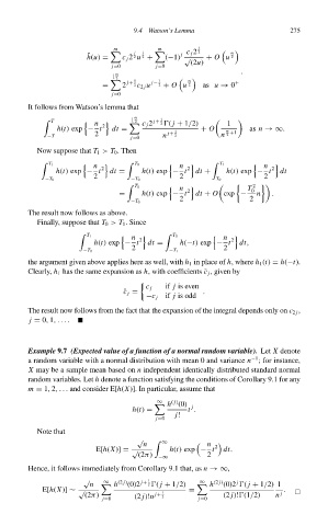
It follows from Watson’s lemma that
m
T n 2 c j 2 j+ 1 2 ( j + 1/2) 1
h(t)exp − t 2 dt = 1 + O m as n →∞.
−T 2 j=0 n j+ 2 n 2 +1
Now suppose that T 1 > T 0 . Then

T 1 n T 0 n T 1 n
h(t)exp − t 2 dt = h(t)exp − t 2 dt + h(t)exp − t 2 dt
2 2 2
−T 0 −T 0 T 0
T 0 n T
2
= h(t)exp − t 2 dt + O exp − 0 n .
2 2
−T 0
The result now follows as above.
Finally, suppose that T 0 > T 1 . Since
n 2 n 2
T 1 T 0

h(t)exp − t dt = h(−t)exp − t dt,
2 2
−T 0 −T 1
the argument given above applies here as well, with h 1 in place of h, where h 1 (t) = h(−t).
Clearly, h 1 has the same expansion as h, with coefficients ¯ c j ,given by

c j if j is even
¯ c j = .
−c j if j is odd
The result now follows from the fact that the expansion of the integral depends only on c 2 j ,
j = 0, 1,....

Example 9.7 (Expected value of a function of a normal random variable). Let X denote
−1
a random variable with a normal distribution with mean 0 and variance n ; for instance,
X may be a sample mean based on n independent identically distributed standard normal
random variables. Let h denote a function satisfying the conditions of Corollary 9.1 for any
m = 1, 2,... and consider E[h(X)]. In particular, assume that
∞ ( j)
h (0) j
h(t) = t .
j!
j=0
Note that
√
n ∞ n 2
E[h(X)] = √ h(t)exp − t dt.
(2π) 2
−∞
Hence, it follows immediately from Corollary 9.1 that, as n →∞,
√ ∞ (2 j) 1 ∞ (2 j) j
n h (0)2 j+ 2 ( j + 1/2) h (0)2 ( j + 1/2) 1
E[h(X)] ∼ √ 1 = j .
(2π) (2 j)!n j+ 2 (2 j)! (1/2) n
j=0 j=0