Page 287 - Elements of Distribution Theory

P1: JZP
052184472Xc09 CUNY148/Severini June 2, 2005 12:8

9.4 Watson’s Lemma 273

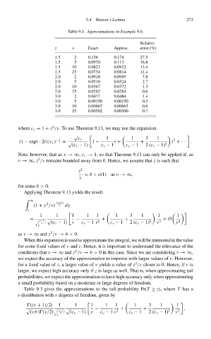
Table 9.3. Approximations in Example 9.6.

Relative
z ν Exact Approx. error (%)

1.5 2 0.136 0.174 27.5
1.5 5 0.0970 0.113 16.8
1.5 10 0.0823 0.0932 13.4
1.5 25 0.0731 0.0814 11.4
2.0 2 0.0918 0.0989 7.8
2.0 5 0.0510 0.0524 2.7
2.0 10 0.0367 0.0372 1.3
2.0 25 0.0282 0.0284 0.6
3.0 2 0.0477 0.0484 1.4
3.0 5 0.00150 0.00150 0.3
3.0 10 0.00667 0.00663 0.6
3.0 25 0.00302 0.00300 0.7

2
where c ν = 1 + z /ν.To use Theorem 9.13, we may use the expansion
√
1 c ν 1 1 3 1 2
(1 − exp(−2t)/c ν ) − 2 = √ 1 − t + + t +· · · .
(c ν − 1) c ν − 1 c ν − 1 2 (c ν − 1) 2
Note, however, that as ν →∞, c ν → 1, so that Theorem 9.13 can only be applied if, as
2
ν →∞, z /ν remains bounded away from 0. Hence, we assume that z is such that
z 2
= b + o(1) as ν →∞,
ν
for some b > 0.
Applying Theorem 9.13 yields the result

∞ −(ν+1)

2
(1 + y /ν) 2 dy
z
1 1 1 1 1 1 3 1 1 1
= √ − + + + O
( ν−1 ) (c ν − 1) ν c ν − 1 ν 2 c ν − 1 2 (c ν − 1) 2 ν 3 ν 4
c ν 2
2
as ν →∞ and z /ν → b > 0.
When this expansion is used to approximate the integral, we will be interested in the value
for some fixed values of ν and z. Hence, it is important to understand the relevance of the
2
conditions that ν →∞ and z /ν → b > 0in this case. Since we are considering ν →∞,
we expect the accuracy of the approximation to improve with larger values of ν.However,
2
for a fixed value of z,a larger value of ν yields a value of z /ν closer to 0. Hence, if ν is
larger, we expect high accuracy only if z is large as well. That is, when approximating tail
probabilities, we expect the approximation to have high accuracy only when approximating
a small probability based on a moderate or large degrees of freedom.
Table 9.3 gives the approximations to the tail probability Pr(T ≥ z), where T has a
t-distribution with ν degrees of freedom, given by

((ν + 1)/2) 1 1 1 1 1 1 3 1 1
√ ν−1 √ − + + ,
(νπ) (ν/2) ( 2 ) (c ν − 1) ν c ν − 1 ν 2 c ν − 1 2 (c ν − 1) 2 ν 3
c ν