Page 136 - Academic Press Encyclopedia of Physical Science and Technology 3rd Chemical Engineering

P1: ZCK/FLS P2: FYK/FLS QC: FYK Revised Pages
Encyclopedia of Physical Science and Technology EN002G-100 May 19, 2001 18:49

758 Chemical Process Design, Simulation, Optimization, and Operation

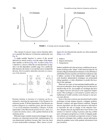
FIGURE 4 (1) Convex and (2) concave functions.

The concept of concave versus convex functions allow niques for one-dimensional searches are often mentioned
us to quantify the behavior of functions analytically (see (Edgar et al., 2001):
Fig. 4).
A single-variable function is convex if the second 1. Indirect
derivative is strictly positive over the range of the depen- 2. Region elimination
dent variable, as shown in Fig. 4(1). As show in Fig. 4(2), 3. Interpolation
a function is concave when the second derivative is neg-
ative over the dependent variable range. For a multivari- Indirect methods solve the necessary conditions for an op-
able function, the matrix of second derivatives (termed the timum (looking at the “shape” of the function) directly via
Hessian, H(x)) is used to check the convexity (or concav- iteration. Region elimination techniques such as Fibonacci
ity) of the function:
and Golden Section searches use function evaluations only
 2 2 2 
∂ f ∂ f ∂ f to delete a portion of the independent variable range at
... each iteration. Interpolation techniques use polynomial
 ∂x 1 2 ∂x 1 ∂x 2 ∂x 1 ∂x n 


 2 2 2  fitting (quadratic or cubic oftentimes) to predict the loca-
 ∂ f ∂ f ∂ f 
...
  tion of the optimum.
2  2 
H(x) =∇ f (x) =  ∂x 2 ∂x 1 ∂x 2 ∂x 2 ∂x n  There are two types of unconstrained multivariable op-
 . . . . 
. . .
 . . . . .  timization techniques: those requiring function derivatives
 
and those that do not. An example of a technique that does
 ∂ f ∂ f 
 2 2 
... ... not require function derivatives is the sequential simplex
∂x n ∂x 1 ∂x 2
n search. This technique is well suited to systems where no
(15) mathematical model currently exists because it uses pro-
cess data directly.
Extrema (minima or maxima) of a function can be ex- Some of the more common unconstrained multivariable
amined by checking the eigenvalues of the Hessian at its techniques include steepest descent, conjugate gradient,
stationary points. If all the eigenvalues of the Hessian are Newton’s method, and quasi-Newton methods. Steepest
positive (negative) at a stationary point, then the function descent algorithms use first-order derivative information
f is at a local minimum (maximum). Likewise, if all the to maximize the rate of change of the objective func-
eigenvalues of the Hessian are positive for all x, then f (x) tion. Steepest descent algorithms have been shown to be
is said to be strictly convex, with a global minimum at the sensitive to function scaling in practice and may exhibit
stationary point. poor convergence properties as a result. Conjugate gradi-
Efficient single-variable numerical techniques for opti- ent methods are essentially an improved version of steep-
mization are important beyond their implementation for est descent techniques that combine current information
one-dimensional problems because they form the basis about the gradient vector with gradient information from
of most multivariable techniques. Three classes of tech- past iterations.