Page 158 - Academic Press Encyclopedia of Physical Science and Technology 3rd Chemical Engineering

P1: LLL Final
Encyclopedia of Physical Science and Technology EN003H-565 June 13, 2001 20:37

220 Coherent Control of Chemical Reactions

Applying W to Eq. (25), we obtain
iH g t 2
iH e
W G (t f ; t 2 , t 1 ) = exp µ ge (R)exp (t f − t 2 )
1 1
h h
(1)
iH e
W X (t) = dt 1 W exp − (t − t 1 ) µ eg (R)

e
h 0 h
iH e
× W G exp − (t f − t 1 ) µ eg (R)

iH e t 1 h
× exp − |X g0 ε(t 1 ). (34)
h

iH g t 1
For a weak field, the probability
W(t) of the wave packet × exp − . (39)
h
existing at the target position at time t is given by
s
(1) 2 (1) (1) Because W in Eq. (39) is a Hermitian operator, the eigen-

W(t) ≈ W X (t) = X (t) W X (t) G

e e e

values λ(t) are real and express the yield of a given target.
1 t f t f
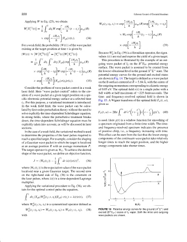
iH g t 2 This procedure is illustrated by the example of an out-
= dt 1 dt 2
X g0 | exp µ ge (R) 3
h 2 0 0 h going wave packet of I 2 on the B 0 potential energy
+
surface. The wave packet is assumed to be created from

iH e iH e 1
+
× exp (t − t 2 ) W exp − (t − t 1 ) µ eg (R) the lowest vibrational level in the ground X state. The
h h
potential energy curves for the ground and excited states
are shown in Fig. 14. The target is defined as a wave packet

iH g t 1
˚
¯
× exp − |X g0 ε(t 2 )ε(t 1 ). (35) on the B surface centered at R = 5.84 A, with the center of
h
the outgoing momentum corresponding to a kinetic energy
Consider the problem of wave packet control in a weak
of 0.05 eV. The optimal field ε(t) is a single pulse with a
laser field. Here “wave packet control” refers to the cre-
full width at half-maximum of ∼225 femtoseconds. The
ation of a wave packet at a given target position on a spe-
time- and frequency-resolved optimal field is shown in
cific electronic potential energy surface at a selected time
Fig. 15. A Wigner transform of the optimal field F w (t,ω),
t f . For this purpose, a variational treatment is introduced.
given as
In the weak field limit, the wave packet can be calcu-
lated by first-order perturbation theory without the need to ∞
t
t
∗

F w (t,ω) = 2Re dt ε t + ε t − g(t ), (40)
solve explicitly the time-dependent Schr¨odinger equation.
0 2 2
In strong fields, where the perturbative treatment breaks
down, the time-dependent Schr¨odinger equation must be is used. Here g(t) is a window function for smoothing of
explicitly taken into account, as will be discussed in later a spectrum originated from a finite time width. The time-
sections. and frequency-resolved spectrum indicates the presence
Inthecaseofaweakfield,thevariationalmethodisused of positive chirp, i.e., a frequency increasing with time.
to determine the properties of the laser pulses required to This effect can be seen from the fact that the lower energy
reach a specified target. For example, consider the shaping components of the continuum wave packet take relatively
of a Gaussian wave packet in which the target is localized longer times to reach the target position, and the higher
¯
¯
at an average position R with an average momentum P. energy components take shorter times.
The target operator is given as W G . To achieve the desired
shape of the wave packet, we define an objective function,
1 t f 2
J =
W G (t f ) − dt λ(t)|ε(t)| , (36)
2 0
where
W G (t f ) istheexpectationvalueofthewavepacket
localized near a given Gaussian target. The second term
on the right-hand side of Eq. (36) is the constraint on
the laser pulses, where λ(t) is a time-dependent Lagrange
multiplier.
Applying the variational procedure to Eq. (36), we ob-
tain for the optimal control pulse the equation,

t f
S
dt 1
X g0 |W (t f ; t, t 1 )|X g0 ε(t 1 ) = λ(t)ε(t), (37)
G
t
S
where W (t f ; t 2 , t 1 ) is a symmetrized operator defined as
G
S 1 +
W (t f ; t 2 , t 1 ) = W G (t f ; t 2 , t 1 ) + W G (t f ; t 1 , t 2 ), (38) FIGURE 14 Potential energy curves for the ground (X ) and
G
3
excited (B 0 +) states of I 2 vapor. Both the initial and outgoing
with wave packets are shown.