Page 159 - Academic Press Encyclopedia of Physical Science and Technology 3rd Chemical Engineering

P1: LLL Final
Encyclopedia of Physical Science and Technology EN003H-565 June 13, 2001 20:37

Coherent Control of Chemical Reactions 221

By varying both ψ(t) → ψ(t) + δψ(t) and ε(t) →
ε(t) + δε(t) in the above equation, the objective function
J is expressed as J + δJ, where δJ has the form

ε(t)

t f
δJ = dt 2Re{i
ξ(t)|µ|ψ(t) } − δε(t)
0 A(t)

t f ∂

+ 2Re dt h ξ(t) δψ(t)

∂t
0

− i
ξ(t)|H(t)|δψ(t) + 2hRe{
ψ(t f )|W|δψ(t f )
−
ξ(t f ) | δψ(t f ) }. (43)
From the optimal condition, δJ = 0, the expression for the
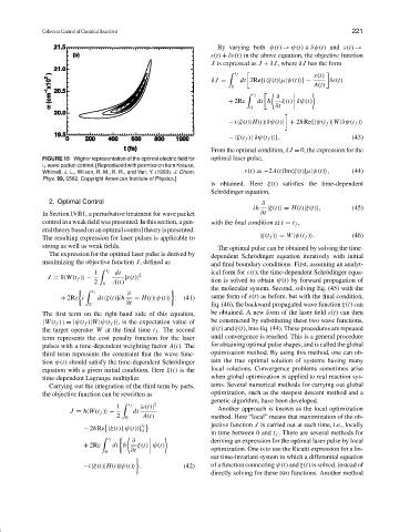
FIGURE 15 Wigner representation of the optimal electric field for optimal laser pulse,
I 2 wave packet control. [Reproduced with permission from Krause,
Whitnell, J. L., Wilson, R. M., K. R., and Yan, Y. (1993). J. Chem. ε(t) =−2A(t)Im
ξ(t)|µ|ψ(t) , (44)
Phys. 99, 6562. Copyright American Institute of Physics.]
is obtained. Here ξ(t) satisfies the time-dependent
Schr¨odinger equation,
2. Optimal Control ∂
ih |ξ(t) = H(t)|ξ(t) , (45)
In Section IVB1, a perturbative treatment for wave packet ∂t
controlinaweakfieldwaspresented.Inthissection,agen- with the final condition at t = t f ,
eraltheorybasedonanoptimalcontroltheoryispresented.
The resulting expression for laser pulses is applicable to |ξ(t f ) = W|ψ(t f ) . (46)
strong as well as weak fields. The optimal pulse can be obtained by solving the time-
The expression for the optimal laser pulse is derived by dependent Schr¨odinger equation iteratively with initial
maximizing the objective function J,defined as and final boundary conditions. First, assuming an analyt-
1 t f dt 2 ical form for ε(t), the time-dependent Schr¨odinger equa-
J = h
W(t f ) − |ε(t)|
2 0 A(t) tion is solved to obtain ψ(t) by forward propagation of
the molecular system. Second, solving Eq. (45) with the

t f ∂
+ 2Re i dt
ξ(t)|ih − H(t)|ψ(t) . (41) same form of ε(t) as before, but with the final condition,
0 ∂t Eq. (46), the backward propagated wave function ξ(t) can
The first term on the right-hand side of this equation, be obtained. A new form of the laser field ε(t) can then

W(t f ) =
ψ(t f )|W|ψ(t f ) , is the expectation value of be constructed by substituting these two wave functions,
the target operator W at the final time t f . The second ψ(t) and ξ(t), into Eq. (44). These procedures are repeated
term represents the cost penalty function for the laser until convergence is reached. This is a general procedure
pulses with a time-dependent weighting factor A(t). The for obtaining optimal pulse shapes, and is called the global
third term represents the constraint that the wave func- optimization method. By using this method, one can ob-
tion ψ(t) should satisfy the time-dependent Schr¨odinger tain the true optimal solution of systems having many
equation with a given initial condition. Here ξ(t)isthe local solutions. Convergence problems sometimes arise
time-dependent Lagrange multiplier. when global optimization is applied to real reaction sys-
Carrying out the integration of the third term by parts, tems. Several numerical methods for carrying out global
the objective function can be rewritten as optimization, such as the steepest descent method and a
genetic algorithm, have been developed.
1 t f |ε(t)| 2 Another approach is known as the local optimization
J = h
W(t f ) − dt
2 0 A(t) method. Here “local” means that maximization of the ob-
jective function J is carried out at each time, i.e., locally
t f

− 2hRe
ξ(t) | ψ(t) | 0
in time between 0 and t f . There are several methods for

t f ∂ deriving an expression for the optimal laser pulse by local

+ 2Re dt h ξ(t) ψ(t)

0 ∂t optimization. One is to use the Ricatti expression for a lin-
ear time-invariant system in which a differential equation

−i
ξ(t)|H(t)|ψ(t) . (42) of a function connecting ψ(t) and ξ(t) is solved, instead of
directly solving for these two functions. Another method