Page 156 - Academic Press Encyclopedia of Physical Science and Technology 3rd Chemical Engineering

P1: LLL Final
Encyclopedia of Physical Science and Technology EN003H-565 June 13, 2001 20:37

218 Coherent Control of Chemical Reactions

(1) (1)
iH e t
X (t) = exp − X (0) , (27)
e e
h
(1)
where X (0) is the nuclear wave packet created on the
e
electronically excited state e just after the delta function
excitation, given by
(1)
iε 0
e
X (0) = µ eg (R)|X g0 . (28)
2h
The time evolution of the wave packet given by Eq. (27)
can be evaluated by an eigenfunction expansion or by
a split-operator technique. With the latter technique, the
(1)
wave packet X (t + δt) after a small increment of time
e
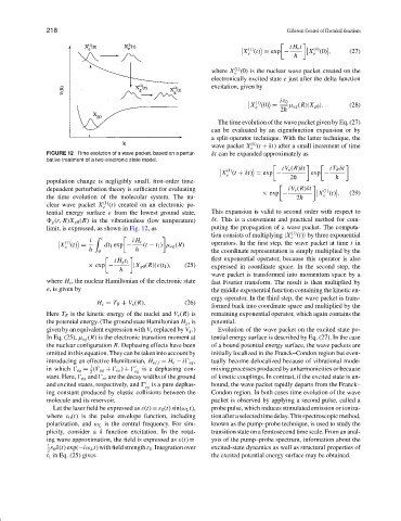
FIGURE 12 Time evolution of a wave packet, based on a pertur- δt can be expanded approximately as
bative treatment of a two-electronic state model.
iV e (R)δt iT R δt

(1)

e
X (t + δt) = exp − exp −
population change is negligibly small, first-order time- 2h h

dependent perturbation theory is sufficient for evaluating iV e (R)δt (1)
× exp − X (t) . (29)
e
the time evolution of the molecular system. The nu- 2h
(1)
clear wave packet X (t) created on an electronic po-
e
tential energy surface e from the lowest ground state, This expansion is valid to second order with respect to
g (r, R)X g0 (R) in the vibrationless (low temperature) δt. This is a convenient and practical method for com-
limit, is expressed, as shown in Fig. 12, as puting the propagation of a wave packet. The computa-
(1)
tion consists of multiplying |X (t) by three exponential
e
i t
(1) operators. In the first step, the wave packet at time t in
iH e
e
X (t) = dt 1 exp − (t − t 1 ) µ eg (R)
h 0 h the coordinate representation is simply multiplied by the
first exponential operator, because this operator is also

iH g t 1
× exp − |X g0 (R) ε(t 1 ), (25) expressed in coordinate space. In the second step, the
h
wave packet is transformed into momentum space by a
where H e , the nuclear Hamiltonian of the electronic state fast Fourier transform. The result is then multiplied by
e,isgivenby the middle exponential function containing the kinetic en-
ergy operator. In the third step, the wave packet is trans-
H e = T R + V e (R). (26)
formed back into coordinate space and multiplied by the
Here T R is the kinetic energy of the nuclei and V e (R)is remaining exponential operator, which again contains the
the potential energy. (The ground state Hamiltonian H g ,is potential.
given by an equivalent expression with V e replaced by V g .) Evolution of the wave packet on the excited state po-
In Eq. (25), µ eg (R) is the electronic transition moment at tential energy surface is described by Eq. (27). In the case
the nuclear configuration R. Dephasing effects have been of a bound potential energy surface, the wave packets are
omitted in this equation. They can be taken into account by initially localized in the Franck–Condon region but even-
introducing an effective Hamiltonian, H ef f = H e − i eg , tually become delocalized because of vibrational mode-
1
in which eg = ( gg + ee ) + is a dephasing con- mixing processes produced by anharmonicities or because
2 eg
stant. Here, gg and ee are the decay widths of the ground of kinetic couplings. In contrast, if the excited state is un-

and excited states, respectively, and is a pure dephas- bound, the wave packet rapidly departs from the Franck–
eg
ing constant produced by elastic collisions between the Condon region. In both cases time evolution of the wave
molecule and its reservoir. packet is observed by applying a second pulse, called a
Let the laser field be expressed as ε(t) = ε 0 (t) sin(ω L t), probe pulse, which induces stimulated emission or ioniza-
where ε 0 (t) is the pulse envelope function, including tionafteraselectedtimedelay.Thisspectroscopicmethod,
polarization, and ω L is the central frequency. For sim- known as the pump–probe technique, is used to study the
plicity, consider a δ function excitation. In the rotat- transition state on a femtosecond time scale. From an anal-
ing wave approximation, the field is expressed as ε(t) = ysis of the pump–probe spectrum, information about the
1 ε 0 δ(t) exp(−iω L t)withfieldstrengthε 0 .Integrationover excited-state dynamics as well as structural properties of
2
t 1 in Eq. (25) gives the excited potential energy surface may be obtained.