Page 350 - Academic Press Encyclopedia of Physical Science and Technology 3rd Analytical Chemistry

P1: GNH/FEE P2: GPJ Final Pages
Encyclopedia of Physical Science and Technology EN010C-493 July 19, 2001 20:30

Nuclear Magnetic Resonance (NMR) 715

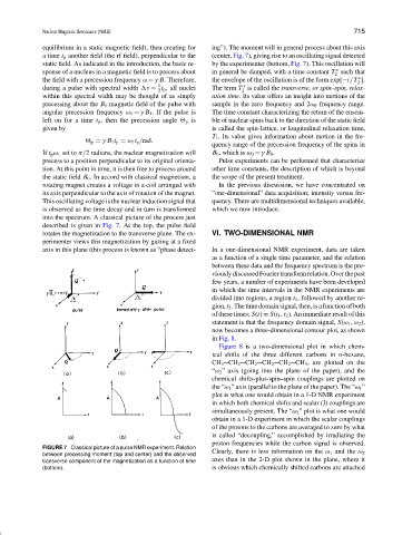
equilibrium in a static magnetic field), then creating for ing”). The moment will in general process about this axis
a time t p another field (the rf field), perpendicular to the (center, Fig. 7), giving rise to an oscillating signal detected
static field. As indicated in the introduction, the basic re- by the experimenter (bottom, Fig. 7). This oscillation will
∗
sponse of a nucleus in a magnetic field is to precess about in general be damped, with a time constant T such that
2
the field with a precession frequency ω = γ B. Therefore, the envelope of the oscillation is of the form exp[−t/T ].
∗
2
1
during a pulse with spectral width ν = t p , all nuclei The term T is called the transverse, or spin–spin, relax-
∗
2 2
within this spectral width may be thought of as simply ation time. Its value offers an insight into motions of the
precessing about the B 1 magnetic field of the pulse with sample in the zero frequency and 2ω 0 frequency range.
angular precession frequency ω 1 = γ B 1 . If the pulse is The time constant characterizing the return of the ensem-
left on for a time t p , then the precession angle p is ble of nuclear spins back to the direction of the static field
given by is called the spin-lattice, or longitudinal relaxation time,
T 1 . Its value gives information about motion in the fre-
p = γ B 1 t p = ω 1 t p /rad.
quency range of the precession frequency of the spins in
If t p ω 1 set to π/2 radians, the nuclear magnetization will B 0 , which is ω 0 = γ B 0 .
precess to a position perpendicular to its original orienta- Pulse experiments can be performed that characterize
tion. At this point in time, it is then free to process around other time constants, the description of which is beyond
the static field B 0 . In accord with classical magnetism, a the scope of the present treatment.
rotating magnet creates a voltage in a coil arranged with In the previous discussion, we have concentrated on
its axis perpendicular to the axis of rotation of the magnet. “one-dimensional” data acquisition; intensity versus fre-
This oscillating voltage is the nuclear induction signal that quency. There are multidimensional techniques available,
is observed as the time decay and in turn is transformed which we now introduce.
into the spectrum. A classical picture of the process just
described is given in Fig. 7. At the top, the pulse field
rotates the magnetization to the transverse plane. The ex- VI. TWO-DIMENSIONAL NMR
perimenter views this magnetization by gazing at a fixed
axis in this plane (this process is known as “phase detect- In a one-dimensional NMR experiment, data are taken
as a function of a single time parameter, and the relation
between these data and the frequency spectrum is the pre-
viously discussed Fourier transform relation. Over the past
few years, a number of experiments have been developed
in which the time intervals in the NMR experiments are
divided into regions, a region t 1 , followed by another re-
gion, t 2 . The time domain signal, then, is a function of both
of these times; S(t) ≡ S(t 1 , t 2 ). An immediate result of this
statement is that the frequency domain signal, S(ω 1 ,ω 2 ),
now becomes a three-dimensional contour plot, as shown
in Fig. 8.
Figure 8 is a two-dimensional plot in which chem-
ical shifts of the three different carbons in n-hexane,
CH 3 CH 2 CH 2 CH 2 CH 2 CH 3 , are plotted on the
“ω 2 ” axis (going into the plane of the paper), and the
chemical shifts-plus-spin–spin couplings are plotted on
the “ω 1 ” axis (parallel to the plane of the paper). The “ω 1 ”
plot is what one would obtain in a 1-D NMR experiment
in which both chemical shifts and scalar (J) couplings are
simultaneously present. The “ω 2 ” plot is what one would
obtain in a 1-D experiment in which the scalar couplings
of the protons to the carbons are averaged to zero by what
is called “decoupling,” accomplished by irradiating the
proton frequencies while the carbon signal is observed.
FIGURE 7 Classical picture of a pulse NMR experiment. Relation
between precessing moment (top and center) and the observed Clearly, there is less information on the ω 1 and the ω 2
transverse component of the magnetization as a function of time axes than in the 2-D plot shown in the plane, where it
(bottom). is obvious which chemically shifted carbons are attached