Page 434 - Engineering Digital Design

404 CHAPTER 9 / PROPAGATION DELAY AND TIMING DEFECTS

(a) (b)
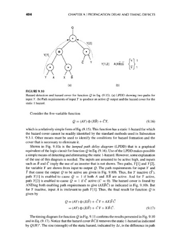
FIGURE 9.10
Hazard detection and hazard cover for function Q in Eq. (9.15). (a) LPDD showing two paths for
input 7. (b) Path requirements of input Y to produce an active Q output and the hazard cover for the
static 1 hazard.

Consider the five-variable function

Q = (AY) 0 (XB) + CY, (9.16)

which is a relatively simple form of Eq. (9.15). This function has a static 1 -hazard for which
the hazard cover cannot be readily identified by the standard methods used in Subsection
9.3.1. Other means must be used to identify the conditions for hazard formation and the
cover that is necessary to eliminate it.
Shown in Fig. 9.10a is the lumped path delay diagram (LPDD) that is a graphical
equivalent of the logic circuit for function Q in Eq. (9.16). Use of the LPDD makes possible
a simple means of detecting and eliminating the static 1-hazard. However, some explanation
of the use of this diagram is needed. The inputs are assumed to be active high, and inputs
such as B and C imply the use of an inverter that is not shown. Two paths, Y[l] and Y[2],
for variable 7 are shown from input to output Q. The path requirements for input Y and
Y that cause the output Q to be active are given in Fig. 9.1 Ob. Thus, for Y inactive (Y),
path Y[l] is enabled to cause Q = 1 if both A and XB are active. And for Y active,
path Y[2] is enabled to cause Q = 1 if C active (C = 0). The hazard cover is found by
ANDing both enabling path requirements to give (AXBC) as indicated in Fig. 9.10b. But
for Y inactive, input A is irrelevant to path K[l]. Thus, the final result for function Q is
given by

Q = (AY) 0 (XB) + CY + AXB C

= (AY)®(XB)+CY+XBC. (9.17)
The timing diagram for function Q in Fig. 9.11 confirms the results presented in Fig. 9.10
and in Eq. (9.17). Notice that the hazard cover BCXremoves the static 1-hazard as indicated
by Q(H)*. The size (strength) of the static hazard, indicated by Af, is the difference in path