Page 545 - Engineering Electromagnetics, 8th Edition

CHAPTER 14 ELECTROMAGNETIC RADIATION AND ANTENNAS 527

P(r,q)

q
r´
q´
(z) r
I s
dz z

z cosq

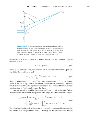
Figure 14.7 A dipole antenna can be represented as a stack of
Hertzian dipoles whose individual phasor currents are given by I s (z).
One Hertzian dipole is shown at location z, and has length dz. When
the observation point, P, lies in the far zone, distance lines r and r
are approximately parallel, so they differ in length by z cos θ.

the distance r from the Hertzian at location z, and the distance r from the origin to

the same point as
.
r = r − z cos θ (54)
.
where, in the far field, θ = θ, and distance lines r and r are approximately parallel.

Eq. (53) is then modified to read
I s (z) kdz
dE θs = j η sin θ e − jk(r−z cos θ) (55)
4πr
.
Notice that in obtaining (55) from (53) we have approximated r = r in the denom-

inator, as the use of Eq. (54) will make little difference when considering amplitude
variations with z and θ. The exponential term in (55) does include (54) because slight
variations in z or θ will greatly impact the phase.
Now, the total electric field at the far-zone position (r,θ) will be the sum of all the
Hertzian dipole contributions along the antenna length, which becomes the integral:
I s (z) kdz

j η sin θ e − jk(r−z cos θ)
E θs (r,θ) = dE θs = 4πr
−
(56)
I 0 k

j η sin θ e − jkr sin k( −|z|) e jkz cos θ dz
=
4πr −
To evaluate the last integral, we first express the complex exponential in terms of sine
and cosine terms using the Euler identity. Denoting the bracketed terms outside the