Page 561 - Engineering Electromagnetics, 8th Edition

CHAPTER 14 ELECTROMAGNETIC RADIATION AND ANTENNAS 543

I 2
I 1
I = –I 2
L
+
V 1 + – Z L V = V L
2
–

Z 11 Z 22
I 1 I L
+
V 1 + – Z I + – Z L V L
21 1
–

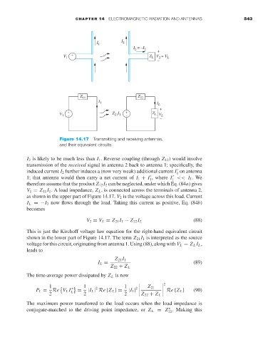
Figure 14.17 Transmitting and receiving antennas,
and their equivalent circuits.

I 2 is likely to be much less than I 1 .Reverse coupling (through Z 12 )would involve
transmission of the received signal in antenna 2 back to antenna 1; specifically, the
induced current I 2 further induces a (now very weak) additional current I on antenna

1
1; that antenna would then carry a net current of I 1 + I , where I << I 1 .We

1
1
therefore assume that the product Z 12 I 2 can be neglected, under which Eq. (84a)gives
V 1 = Z 11 I 1 .A load impedance, Z L ,is connected across the terminals of antenna 2,
as shown in the upper part of Figure 14.17. V 2 is the voltage across this load. Current
I L =−I 2 now flows through the load. Taking this current as positive, Eq. (84b)
becomes
(88)
V 2 = V L = Z 21 I 1 − Z 22 I L
This is just the Kirchoff voltage law equation for the right-hand equivalent circuit
shown in the lower part of Figure 14.17. The term Z 21 I 1 is interpreted as the source
voltage for this circuit, originating from antenna 1. Using (88), along with V L = Z L I L ,
leads to

Z 21 I 1
I L = (89)
Z 22 + Z L
The time-average power dissipated by Z L is now

1 1 1 Z 21 2
2
P L = Re V L I L ∗ = |I L | Re {Z L } = |I 1 | 2 Re {Z L } (90)
2 2 2 Z 22 + Z L
The maximum power transferred to the load occurs when the load impedance is
conjugate-matched to the driving point impedance, or Z L = Z . Making this
∗
22