Page 107 - Essentials of applied mathematics for scientists and engineers

book Mobk070 March 22, 2007 11:7

INTEGRAL TRANSFORMS: THE LAPLACE TRANSFORM 97
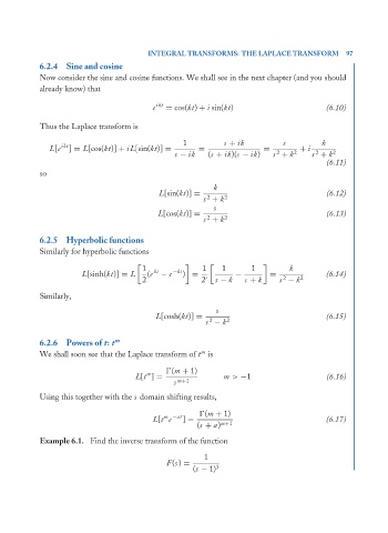
6.2.4 Sine and cosine
Now consider the sine and cosine functions. We shall see in the next chapter (and you should
already know) that

e ikt = cos(kt) + i sin(kt) (6.10)

Thus the Laplace transform is

1 s + ik s k
L[e ikt ] = L[cos(kt)] + iL[sin(kt)] = = = + i
s − ik (s + ik)(s − ik) s + k 2 s + k 2
2
2
(6.11)
so
k
L[sin(kt)] = (6.12)
2
s + k 2
s
L[cos(kt)] = (6.13)
2
s + k 2
6.2.5 Hyperbolic functions
Similarly for hyperbolic functions

1 1 1 1 k

kt
L[sinh(kt)] = L (e − e −kt ) = − = (6.14)
2
2 2 s − k s + k s − k 2
Similarly,
s
L[cosh(kt)] = (6.15)
2
s − k 2
6.2.6 Powers of t: t m
m
We shall soon see that the Laplace transform of t is
(m + 1)
m
L[t ] = m > −1 (6.16)
s m+1
Using this together with the s domain shifting results,
(m + 1)
m −at
L[t e ] = (6.17)
(s + a) m+1
Example 6.1. Find the inverse transform of the function

1
F(s ) =
(s − 1) 3