Page 469 - Excel 2007 Bible

27_044039 ch21.qxp 11/21/06 11:12 AM Page 426
Part III
Creating Charts and Graphics
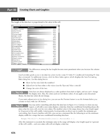
FIGURE 21.4
The length of the data bars is proportional to the value in the cell.
TIP The differences among the bar lengths become more prominent when you increase the column
TIP
width.
Excel provides quick access to six data bar colors via the Home ➪ Styles ➪ Conditional Formatting ➪ Data
Bars command. For additional choices, click the More Rules option, which displays the New Formatting
Rule dialog box. Use this dialog box to:
n Show the bar only (hide the numbers)
n Adjust how the bars relate to the values (use the Type and Value controls)
n Change the color of the bars
NOTE Data bars are always displayed as a color gradient (from dark to light), and you can’t change
NOTE
the display style. Also, the colors used are not theme colors. If you apply a new document
theme, the data bar colors do not change.
If you make adjustments in this dialog box, you can use the Preview button to see the formats before you
commit to them with the OK button.
NOTE You may notice something odd about the data bars in Figure 21.4. Contrary to what you may
NOTE
expect, a cell with a zero value displays a data bar. Data bar conditional formatting always dis-
plays a bar for every cell, even for zero values. The smallest value in the range always has a bar length equal
to 10 percent of the cell’s width. Unfortunately, Excel provides no direct way to modify the minimum per-
cent setting. But, if you’re familiar with VBA, you can use a statement like the following to set the minimum
display width for a range that uses conditional formatting data bars:
Range(“B2:B123”).FormatConditions(1).PercentMin = 1
After this statement is executed, the minimum value in the range will display a bar length equal to 1 percent
of the cell’s width — and zero value cells will not display a data bar.

426