Page 477 - Excel 2007 Bible

27_044039 ch21.qxp 11/21/06 11:12 AM Page 434
Part III
Creating Charts and Graphics
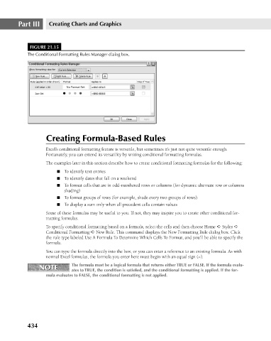
FIGURE 21.15
The Conditional Formatting Rules Manager dialog box.
Creating Formula-Based Rules
Excel’s conditional formatting feature is versatile, but sometimes it’s just not quite versatile enough.
Fortunately, you can extend its versatility by writing conditional formatting formulas.
The examples later in this section describe how to create conditional formatting formulas for the following:
n To identify text entries
n To identify dates that fall on a weekend
n To format cells that are in odd-numbered rows or columns (for dynamic alternate row or columns
shading)
n To format groups of rows (for example, shade every two groups of rows).
n To display a sum only when all precedent cells contain values
Some of these formulas may be useful to you. If not, they may inspire you to create other conditional for-
matting formulas.
To specify conditional formatting based on a formula, select the cells and then choose Home ➪ Styles ➪
Conditional Formatting ➪ New Rule. This command displays the New Formatting Rule dialog box. Click
the rule type labeled Use A Formula To Determine Which Cells To Format, and you’ll be able to specify the
formula.
You can type the formula directly into the box, or you can enter a reference to an existing formula. As with
normal Excel formulas, the formula you enter here must begin with an equal sign (=).

NOTE The formula must be a logical formula that returns either TRUE or FALSE. If the formula evalu-
NOTE
ates to TRUE, the condition is satisfied, and the conditional formatting is applied. If the for-
mula evaluates to FALSE, the conditional formatting is not applied.

434