Page 480 - Excel 2007 Bible

27_044039 ch21.qxp 11/21/06 11:12 AM Page 437
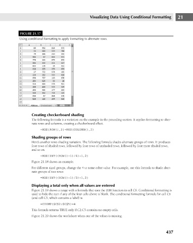
FIGURE 21.17
Using conditional formatting to apply formatting to alternate rows.
Creating checkerboard shading Visualizing Data Using Conditional Formatting 21
The following formula is a variation on the example in the preceding section. It applies formatting to alter-
nate rows and columns, creating a checkerboard effect.
=MOD(ROW(),2)=MOD(COLUMN(),2)

Shading groups of rows
Here’s another rows shading variation. The following formula shades alternate groups of rows. It produces
four rows of shaded rows, followed by four rows of unshaded rows, followed by four more shaded rows,
and so on.
=MOD(INT((ROW()-1)/4)+1,2)
Figure 21.18 shows an example.
For different sized groups, change the 4 to some other value. For example, use this formula to shade alter-
nate groups of two rows:
=MOD(INT((ROW()-1)/2)+1,2)
Displaying a total only when all values are entered
Figure 21.19 shows a range with a formula that uses the SUM function in cell C6. Conditional formatting is
used to hide the sum if any of the four cells above is blank. The conditional formatting formula for cell C6
(and cell C5, which contains a label) is

=COUNT($C$2:$C$5)=4
This formula returns TRUE only if C2:C5 contains no empty cells.
Figure 21.20 shows the worksheet when one of the values is missing.

437