Page 479 - Excel 2007 Bible

27_044039 ch21.qxp 11/21/06 11:12 AM Page 436
Part III
Creating Charts and Graphics
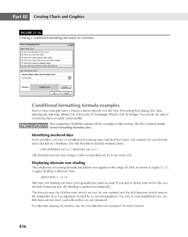
FIGURE 21.16
Creating a conditional formatting rule based on a formula.
Conditional formatting formula examples
Each of these examples uses a formula entered directly into the New Formatting Rule dialog box, after
selecting the rule type labeled Use A Formula To Determine Which Cells To Format. You decide the type of
formatting that you apply conditionally.
ON the CD-ROM The companion CD-ROM contains all the examples in this section. The file is named condi-
ON the CD-ROM
tional formatting formulas.xlsx.
Identifying weekend days
Excel provides a number of conditional formatting rules that deal with dates, but it doesn’t let you identify
dates that fall on a weekend. Use this formula to identify weekend dates:
=OR(WEEKDAY(A1)=7,WEEKDAY(A1)=1)
This formula assumes that a range is selected and that cell A1 is the active cell.

Displaying alternate-row shading
The conditional formatting formula that follows was applied to the range A1:D18, as shown in Figure 21.17,
to apply shading to alternate rows.
=MOD(ROW(),2)=0
Alternate row shading can make your spreadsheets easier to read. If you add or delete rows within the con-
ditional formatting area, the shading is updated automatically.
This formula uses the ROW function (which returns the row number) and the MOD function (which returns
the remainder of its first argument divided by its second argument). For cells in even-numbered rows, the
MOD function returns 0, and cells in that row are formatted.
For alternate shading of columns, use the COLUMN function instead of the ROW function.

436