Page 196 - Excel Workbook for Dummies

20_798452 ch14.qxp 3/13/06 7:50 PM Page 179
Chapter 14: Charting Spreadsheet Data 179
Note that data labels identify the various data series in a chart either with the
data series names (the part numbers in this case), category names (the dates),
or values.
13. Click the Data Table tab and then select the Show Data Table check box.
Excel draws a data table in the preview right below the preview of the Clustered
Bar chart. This table shows all the values that are graphed in the chart. Adding a
data table to chart that you place on a separate chart sheet is sometimes an
effective way to include the underlying data in chart’s printout.
14. Remove the check mark from the Show Data Table check box and then select the
Next button.
The Chart Wizard –Step 4 of 4 – Chart Locations dialog box, where you can
choose between embedding the new chart in the worksheet as a graphic object
(the default) or on a new sheet, appears.
15. Leave the As Object In option button with the Sales-06 worksheet selected as you
select the Finish button.
16. Move the chart so that its top edge is flush with the top edge of row 17 and its
left edge is flush with the left edge of column E before you resize the chart so
that its bottom edge is flush with the bottom edge of row 35 and its right edge
flush with the right edge of column R.
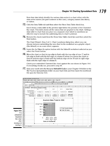
Check your embedded Clustered Bar chart against the one shown in Figure 14-6.
If everything checks out, proceed to step 18.
17. Save your work with the filename Solved14-2.xls in your Chapter 14 folder in the
My Practice Spreadsheets folder on your hard disk and then leave the workbook
file open for Exercise 14-3.

Figure 14-6:
The
embedded
Clustered
Bar chart
after
moving and
resizing it.