Page 194 - Excel Workbook for Dummies

20_798452 ch14.qxp 3/13/06 7:49 PM Page 177
Chapter 14: Charting Spreadsheet Data 177

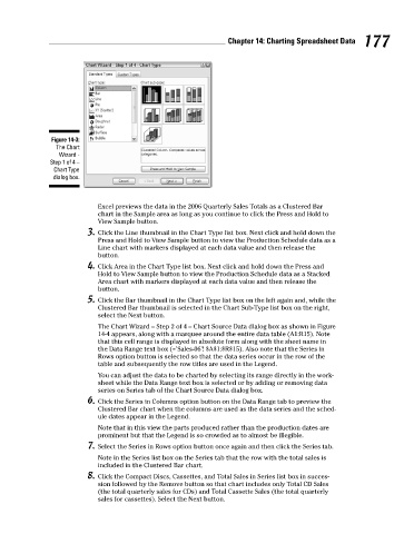
Figure 14-3:
The Chart
Wizard -
Step 1 of 4 –
Chart Type
dialog box.

Excel previews the data in the 2006 Quarterly Sales Totals as a Clustered Bar
chart in the Sample area as long as you continue to click the Press and Hold to
View Sample button.

3. Click the Line thumbnail in the Chart Type list box. Next click and hold down the
Press and Hold to View Sample button to view the Production Schedule data as a
Line chart with markers displayed at each data value and then release the
button.
4. Click Area in the Chart Type list box. Next click and hold down the Press and
Hold to View Sample button to view the Production Schedule data as a Stacked
Area chart with markers displayed at each data value and then release the
button.
5. Click the Bar thumbnail in the Chart Type list box on the left again and, while the
Clustered Bar thumbnail is selected in the Chart Sub-Type list box on the right,
select the Next button.
The Chart Wizard – Step 2 of 4 – Chart Source Data dialog box as shown in Figure
14-4 appears, along with a marquee around the entire data table (A1:R15). Note
that this cell range is displayed in absolute form along with the sheet name in
the Data Range text box (=’Sales-06’! $A$1:$R$15). Also note that the Series in
Rows option button is selected so that the data series occur in the row of the
table and subsequently the row titles are used in the Legend.
You can adjust the data to be charted by selecting its range directly in the work-
sheet while the Data Range text box is selected or by adding or removing data
series on Series tab of the Chart Source Data dialog box.
6. Click the Series in Columns option button on the Data Range tab to preview the
Clustered Bar chart when the columns are used as the data series and the sched-
ule dates appear in the Legend.
Note that in this view the parts produced rather than the production dates are
prominent but that the Legend is so crowded as to almost be illegible.
7. Select the Series in Rows option button once again and then click the Series tab.
Note in the Series list box on the Series tab that the row with the total sales is
included in the Clustered Bar chart.
8. Click the Compact Discs, Cassettes, and Total Sales in Series list box in succes-
sion followed by the Remove button so that chart includes only Total CD Sales
(the total quarterly sales for CDs) and Total Cassette Sales (the total quarterly
sales for cassettes). Select the Next button.