Page 311 - Excel for Scientists and Engineers: Numerical Methods

288 EXCEL: NUMERICAL METHODS

y = ae" (13-2)

Least-Squares Fit to a Straight Line

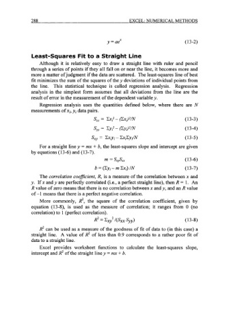
Although it is relatively easy to draw a straight line with ruler and pencil
through a series of points if they all fall on or near the line, it becomes more and
more a matter of judgment if the data are scattered. The least-squares line of best
fit minimizes the sum of the squares of the y deviations of individual points from
the line. This statistical technique is called regression analysis. Regression
analysis in the simplest form assumes that all deviations from the line are the
result of error in the measurement of the dependent variable y.
Regression analysis uses the quantities defined below, where there are N
measurements of xi, yi data pairs.
S,, = CX,~ (CXJ2/N (1 3-3)
-
Syy = Cy,2 - (CyJ2/N (1 3-4)

Sxy = CX$~ - CxiCyi/N (13-5)
For a straight line y = mx + by the least-squares slope and intercept are given
by equations (13-6) and (13-7).
m = SX,& (1 3-6)
b = (Cy, - m Cx,) lN (1 3-7)

The Correlation coefficient, R, is a measure of the correlation between x and
y. If x and y are perfectly correlated (i.e., a perfect straight line), then R = 1. An
R value of zero means that there is no correlation between x and y, and an R value
of -1 means that there is a perfect negative correlation.
More commonly, R2, the square of the correlation coefficient, given by
equation (13-S), is used as the measure of correlation; it ranges from 0 (no
correlation) to 1 (perfect correlation).

R2 = Cv2 l(Sxx Syy) (13-8)
R2 can be used as a measure of the goodness of fit of data to (in this case) a
straight line. A value of R2 of less than 0.9 corresponds to a rather poor fit of
data to a straight line.
Excel provides worksheet functions to calculate the least-squares slope,
intercept and R2 of the straight line y = mx + b.