Page 316 - Excel for Scientists and Engineers: Numerical Methods

CHAPTER 13 LINEAR REGRESSION AND CURVE FITTING 293

Type the LINEST formula with its arguments, in this example
=LINEST(F3:F14,E3: E14,TRUE,TRUE). You can use the following
"shorthand" for the logical arguments const and stats: FALSE can be
represented by 0 and TRUE by any nonzero value, as in the formula
=LINEST(F3:F14,E3:E14,1,1).
Enter the formula by using CONTROL+SHIFT+ENTER.
When you "array-enter" a formula, Excel puts braces around the formula, as
shown below:
{=LINEST(F3:F14,E3:E14,1,1)}

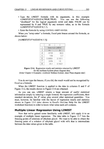
Figure 13-6. Regression results and statistics returned by LINEST
for the methane hydrate phase diagram data.
(folder 'Chapter 13 Examples', workbook 'Methane Hydrate', sheet 'Phase diagram data')

You do not type the braces; if you did, the result would not be recognized by
Excel as a formula.
When the LINEST function is applied to the data in columns E and F of
Figure 13-2, the results shown in Figure 13-6 are obtained.
As you can see, LINEST returns a large amount of useful statistical
information simply by entering a single formula: the regression coefficients, their
standard deviations, the R2 value, plus several other statistical quantities. You
must, however, be familiar with the layout of regression results and statistics
shown in Figure 13-5 (also shown in Excel's On-Line Help for the LINEST
worksheet function) in order to know what value each cell contains.

Multiple Linear Regression Using LINEST
Now that we've gained some familiarity with LINEST, let's apply it to an
example of multiple linear regression. The data table in Figure 13-7 lists the
freezing points of solutions of ethylene glycol. We want to be able to obtain the
freezing point of a solution of ethylene glycol with wt% that is intermediate
between the data values given in the table.