Page 319 - Excel for Scientists and Engineers: Numerical Methods

296 EXCEL: NUMERICAL METHODS

four regression coefficients) and up to five rows deep (LINEST can return five
rows of regression statistics, as illustrated in Figure 13-5). If you want to see the
curve-fitting coefficients, their standard deviations and the R2 value, you need
only select a range that is three rows deep.
Third, enter the LINEST formula with its arguments:
=LI N EST(D2: D14,A2:C14,1,1)

Finally, enter the array function by pressing CONTROL+SHIFT+ENTER
(Windows) or CONTROL+SHIFT+RETURN (Macintosh).
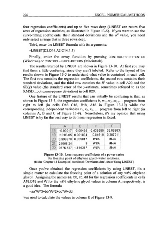
The results returned by LINEST are shown in Figure 13-10. At first you may
find them a little confusing, since they aren't labeled. Refer to the layout of the
results shown in Figure 13-5 to understand what value is contained in each cell.
The first row contains the regression coefficients, the second row contains their
standard deviations, and the third row contains the R2 value in cell A20 and the
SE(y) value (the standard error of the y-estimate, sometimes referred to as the
RMSD, root-mean-square deviation) in cell B20.
One feature of the LINEST results that can initially be confusing is that, as
shown in Figure 13-5, the regression coefficients by ml, m2, m3 ,. . . progress from
right to left (in cells D18 C18, B18, A18 in Figure 13-10) while the
corresponding independent variables xl, x2, x3, ... progress from left to right (in
columns A, B and C of Figure 13-9). Nonetheless, it's my opinion that using
LINEST is by far the best way to do linear regression in Excel.

Figure 13-10. Least-squares coefficients of a power series
for freezing point of ethylene glycol-water solutions.
(folder 'Chapter 13 Examples', workbook 'Dowtherm data', sheet 'Using LINEST')
Once you've obtained the regression coefficients by using LINEST, it's a
simple matter to calculate the freezing point of a solution of any wtY0 ethylene
glycol. Assigning the names aa, bb, cc, dd for the regression coefficients in cells
A1 8: D18 and W for the wt% ethylene glycol values in column A, respectively, is
a good idea. The formula
=aa*WA3+ bb*WA2+cc*W+dd
was used to calculate the values in column E of Figure 13-9.