
Page 322 - Excel for Scientists and Engineers: Numerical Methods
P. 322
CHAPTER 13 LINEAR REGRESSION AND CURVE FITTING 299
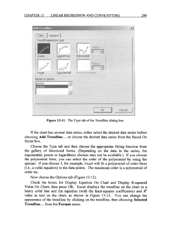
Figure 13-11. The Type tab of the Trendline dialog box.
If the chart has several data series, either select the desired data series before
choosing Add Trendline ... or choose the desired data series from the Based On
Series box.
Choose the Type tab and then choose the appropriate fitting function from
the gallery of hnctional forms. (Depending on the data in the series, the
exponential, power or logarithmic choices may not be available.) If you choose
the polynomial form, you can select the order of the polynomial by using the
spinner. If you choose 3, for example, Excel will fit a polynomial of order three
(i.e., a cubic equation) to the data points. The maximum order is a polynomial of
order six.
Now choose the Options tab (Figure 13-12).
Check the boxes for Display Equation On Chart and Display R-squared
Value On Chart; then press OK. Excel displays the trendline on the chart as a
heavy solid line and the equation (with the least-squares coefficients) and k
value as text on the chart, as shown in Figure 13-13. You can change the
appearance of the trendline by clicking on the trendline, then choosing Selected
Trendline.. . from the Format menu.