Page 317 - Excel for Scientists and Engineers: Numerical Methods

294 EXCEL: NUMERICAL METHODS

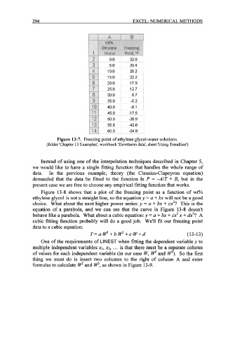
Figure 13-7. Freezing point of ethylene glycol-water solutions.
(folder 'Chapter 13 Examples', workbook 'Dowtherm data', sheet 'Using Trendline')

Instead of using one of the interpolation techniques described in Chapter 5,
we would like to have a single fitting function that handles the whole range of
data. In the previous example, theory (the Clausius-Clapeyron equation)
demanded that the data be fitted to the function In P = -A/T + B, but in the
present case we are free to choose any empirical fitting function that works.
Figure 13-8 shows that a plot of the freezing point as a function of wt%
ethylene glycol is not a straight line, so the equation y = a + bx will not be a good
choice. What about the next higher power series: y = a + bx + cx2? This is the
equation of a parabola, and we can see that the curve in Figure 13-8 doesn't
behave like a parabola. What about a cubic equation: y = a + bx + cx2 x + ak3? A
cubic fitting function probably will do a good job. We'll fit our freezing point
data to a cubic equation:
T=a.W3 + b.W2 +c.W+d (1 3-13)
One of the requirements of LINEST when fitting the dependent variable y to
multiple independent variables XI, x2, . . . is that there must be a separate column
of values for each independent variable (in our case W, W2 and W3). So the first
thing we must do is insert two columns to the right of column A and enter
formulas to calculate W2 and P, as shown in Figure 13-9.