Page 287 - Fair, Geyer, and Okun's Water and wastewater engineering : water supply and wastewater removal

JWCL344_ch07_230-264.qxd 8/2/10 8:44 PM Page 247

7.7 Automated Optimization 247

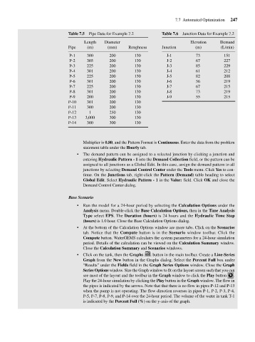
Table 7.5 Pipe Data for Example 7.2 Table 7.6 Junction Data for Example 7.2

Length Diameter Elevation Demand
Pipe (m) (mm) Roughness Junction (m) (L/min)
P-1 300 200 130 J-1 73 151
P-2 305 200 130 J-2 67 227
P-3 225 200 130 J-3 85 229
P-4 301 200 130 J-4 61 212
P-5 225 200 130 J-5 82 208
P-6 301 200 130 J-6 56 219
P-7 225 200 130 J-7 67 215
P-8 301 200 130 J-8 73 219
P-9 200 200 130 J-9 55 215
P-10 301 200 130
P-11 300 200 130
P-12 1 250 130
P-13 3,000 300 130
P-14 300 300 130

Multiplier is 0.80, and the Pattern Format is Continuous. Enter the data from the problem
statement table under the Hourly tab.
• The demand pattern can be assigned to a selected junction by clicking a junction and
entering Hydraulic Pattern - 1 into the Demand Collection field, or the pattern can be
assigned to all junctions as a Global Edit. In this case, assign the demand pattern to all
junctions by selecting Demand Control Center under the Tools menu. Click Yes to con-
tinue. On the Junctions tab, right-click the Pattern (Demand) table heading to select
Global Edit. Select Hydraulic Pattern - 1 in the Value: field. Click OK and close the
Demand Control Center dialog.

Base Scenario
• Run the model for a 24-hour period by selecting the Calculation Options under the
Analysis menu. Double-click the Base Calculation Options, then in the Time Analysis
Type select EPS. The Duration (hours) is 24 hours and the Hydraulic Time Step
(hours) is 1.0 hour. Close the Base Calculation Options dialog.
• At the bottom of the Calculation Options window are more tabs. Click on the Scenarios
tab. Notice that the Compute button is in the Scenario window toolbar. Click the
Compute button. WaterGEMS calculates the system parameters for a 24-hour simulation
period. Details of the calculation can be viewed on the Calculation Summary window.
Close the Calculation Summary and Scenarios windows.
• Click on the tank, then the Graphs button in the main toolbar. Create a Line-Series
Graph from the New button in the Graphs dialog. Select the Percent Full box under
“Results” under the Fields field in the Graph Series Options window. Close the Graph
Series Options window. Size the Graph window to fit on the layout screen such that you can
see most of the layout and the toolbar in the Graph window to click the Play button .
Play the 24-hour simulation by clicking the Play button in the Graph window. The flow in
the pipes is indicated by the arrows. Note that that there is no flow in pipes P-12 and P-13
when the pump is not operating. The flow direction reverses in pipes P-1, P-2, P-3, P-4,
P-5, P-7, P-8, P-9, and P-14 over the 24-hour period. The volume of the water in tank T-1
is indicated by the Percent Full (%) on the y-axis of the graph.