Page 291 - Fair, Geyer, and Okun's Water and wastewater engineering : water supply and wastewater removal

JWCL344_ch07_230-264.qxd 8/2/10 8:44 PM Page 251

7.7 Automated Optimization 251

Chlorine concentration

0.900
0.800
Concentration (mg/L) 0.600
0.700

0.500
0.400
0.300
0.200
0.100
0.000
0.000 24.000 48.000 72.000 96.000 120.000 144.000 168.000
Time (hours)
T-1 J-7 J-2 J-9 J-3

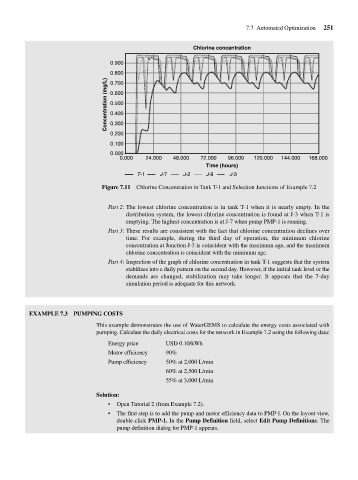
Figure 7.11 Chlorine Concentration in Tank T-1 and Selection Junctions of Example 7.2

Part 2: The lowest chlorine concentration is in tank T-1 when it is nearly empty. In the
distribution system, the lowest chlorine concentration is found at J-3 when T-1 is
emptying. The highest concentration is at J-7 when pump PMP-1 is running.
Part 3: These results are consistent with the fact that chlorine concentration declines over
time. For example, during the third day of operation, the minimum chlorine
concentration at Junction J-3 is coincident with the maximum age, and the maximum
chlorine concentration is coincident with the minimum age.
Part 4: Inspection of the graph of chlorine concentration in tank T-1 suggests that the system
stabilizes into a daily pattern on the second day. However, if the initial tank level or the
demands are changed, stabilization may take longer. It appears that the 7-day
simulation period is adequate for this network.

EXAMPLE 7.3 PUMPING COSTS
This example demonstrates the use of WaterGEMS to calculate the energy costs associated with
pumping. Calculate the daily electrical costs for the network in Example 7.2 using the following data:
Energy price USD 0.10/kWh
Motor efficiency 90%
Pump efficiency 50% at 2,000 L/min
60% at 2,500 L/min
55% at 3,000 L/min

Solution:
• Open Tutorial 2 (from Example 7.2).
• The first step is to add the pump and motor efficiency data to PMP-l. On the layout view,
double-click PMP-1. In the Pump Definition field, select Edit Pump Definitions. The
pump definition dialog for PMP-1 appears.