Page 53 - Finite Element Analysis with ANSYS Workbench

44 Chapter 3 Beam Analysis

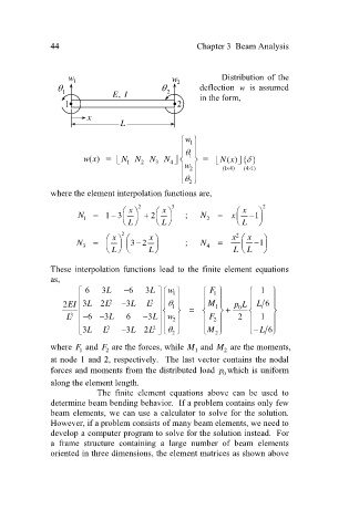
w 1 w Distribution of the
 1 , EI  2 2 deflection w is assumed

1 2 in the form,
x
L

 w 1 
  
1 

wx 1  2 N N   3 4     Nx    ()   
()  NN

 w 2  (1 4) (4 1)


  
2 

where the element interpolation functions are,
3 2
2


N  13   x    2   x   ; N  x   x  1

1
 L   L  2  L 


N    x   2   32 x   ; N  x  2  x  1

3

 L   L  4 LL 

These interpolation functions lead to the finite element equations
as,
6  3 L 6  3 L   w 1  F  1  1  
 3 2EI 2L 2   3 L L L 2            M  1      pL  0   6 L   
1
L 3 6   3  6 L 3  L  w 2  F 2   2  1 
      M  
 3 2  3L L 2 L L  2  2 2    L   6  
where F and F are the forces, while M and M are the moments,
2
1
1
2
at node 1 and 2, respectively. The last vector contains the nodal
forces and moments from the distributed load p which is uniform
0
along the element length.
The finite element equations above can be used to
determine beam bending behavior. If a problem contains only few
beam elements, we can use a calculator to solve for the solution.
However, if a problem consists of many beam elements, we need to
develop a computer program to solve for the solution instead. For
a frame structure containing a large number of beam elements
oriented in three dimensions, the element matrices as shown above