Page 287 - Finite Element Modeling and Simulations with ANSYS Workbench

272 Finite Element Modeling and Simulation with ANSYS Workbench

The response of each mode Z is similar to that of a single DOF system. Once the natural
i
coordinate vector z is known, we can recover the real displacement vector u from z using
Equation 8.24.

8.4.2 Direct Method
In this approach, we solve Equation 8.27 directly, that is, compute the inverse of the coef-
ficient matrix, which is in general much more expensive than the modal method.
ω
Using complex notation to represent the harmonic response, we have u = ue and
it
Equation 8.27 becomes:
] =
i
[K +ω C −ω 2 Mu F (8.30)
Inverting the matrix [K +ωi C −ω 2 M ], we can obtain the displacement amplitude
vector u. However, this equation is expensive to solve for large systems and the matrix
[K +ω C −ω 2 M ] can become ill-conditioned if ω is close to any natural frequency ω of the
i
i
structure. Therefore, the direct method is only applied when the system of equations is
small and the frequency is away from any natural frequency of the structure.

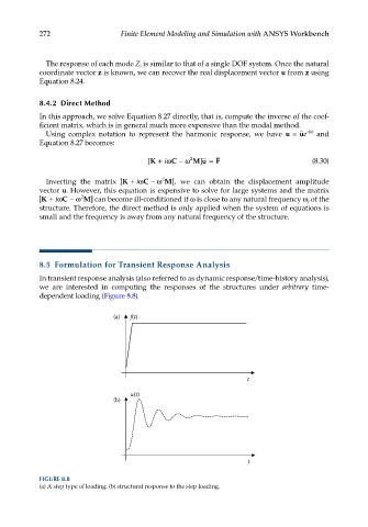
8.5 Formulation for Transient Response Analysis

In transient response analysis (also referred to as dynamic response/time-history analysis),
we are interested in computing the responses of the structures under arbitrary time-
dependent loading (Figure 8.8).

(a) f(t)

t

u(t)
(b)

t

FIGURE 8.8
(a) A step type of loading; (b) structural response to the step loading.