Page 288 - Finite Element Modeling and Simulations with ANSYS Workbench

Structural Vibration and Dynamics 273

u(t)
u 1

u k u k + 1
u 2

t 0 t 1 t 2 t k t k + 1 t

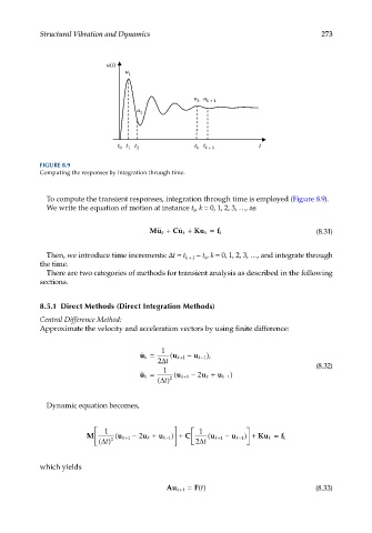
FIGURE 8.9
Computing the responses by integration through time.

To compute the transient responses, integration through time is employed (Figure 8.9).
We write the equation of motion at instance t , k = 0, 1, 2, 3, …, as
k

Mu + Cu + Ku k = (8.31)
k k f k

Then, we introduce time increments: Δt = t k + 1 − t , k = 0, 1, 2, 3, …, and integrate through
k
the time.
There are two categories of methods for transient analysis as described in the following
sections.

8.5.1 Direct Methods (Direct Integration Methods)
Central Difference Method:
Approximate the velocity and acceleration vectors by using finite difference:

1
u k = ( u k+1 − u k−1 ),
2∆ t (8.32)
1
u k = 2 ( u k+1 − 2 u k + u k−1 )
t ∆ ()

Dynamic equation becomes,

 1   1 
1 ) +
M  2 u ( k+ 1 − 2 u k + u k−  C  u ( k+ 1 − u k− 1 ) + Ku k = f k

∆
t
 ()   2∆t 
which yields

Au k+ = F t() (8.33)
1