Page 283 - Finite Element Modeling and Simulations with ANSYS Workbench

268 Finite Element Modeling and Simulation with ANSYS Workbench

This is a generalized eigenvalue problem (EVP). The trivial solution is u = 0 for any val-
ues of ω (not interesting). Nontrivial solutions (u ≠ ) 0 exist only if:

K −ω 2 M = 0 (8.18)

This is an n-th order polynomial of ω , from which we can find n solutions (roots) or
2
eigenvalues ω (i = 1, 2, …, n). These are the natural frequencies (or characteristic frequen-
i
cies) of the structure.
The smallest nonzero eigenvalue ω is called the fundamental frequency.
1
For each ω , Equation 8.17 gives one solution or eigen vector:
i
2 M ]u = 0
[K −ω i i
u i (i = 1, 2, …, n) are the normal modes (or natural modes, mode shapes, and so on).

Properties of the Normal Modes:
Normal modes satisfy the following properties:

T
T
uKu j = 0, u Mu j = 0, for i ≠ j (8.19)
i i
if ω i ≠ ω j . That is, modes are orthogonal (thus independent) to each other with respect to K
and M matrices.
Normal modes are usually normalized:

T
T
uMu i = 1, u Ku i = ω 2 (8.20)
i i i
Notes:
• Magnitudes of displacements (modes) or stresses in normal mode analysis have
no physical meaning.
• For normal mode analysis, no support of the structure is necessary.
• ω = 0 means there are rigid-body motions of the whole or a part of the structure.
i
This can be applied to check the FEA model (check to see if there are mechanisms
or free elements in the FEA models).
• Lower modes are more accurate than higher modes in the FEA calculations (due
to less spatial variations in the lower modes leading to that fewer elements/wave-
lengths are needed).

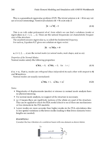
EXAMPLE 8.1
Consider the free vibration of a cantilever beam with one element as shown below.
y
v 2
, A, EI 2
1 2 x
L