Page 353 - Finite Element Modeling and Simulations with ANSYS Workbench

338 Finite Element Modeling and Simulation with ANSYS Workbench

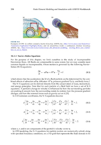
FIGURE 10.1
Examples of CFD: (a) airflow around a tractor (Courtesy ANSYS, Inc., http://www.ansys.com/Industries/
Automotive/Application+Highlights/Body), and (b) streamlines inside a combustion chamber (Courtesy
ANSYS, Inc., http://www.edr.no/en/courses/ansys_cfd_advanced_modeling_ reacting_flows_and_combus-
tion_in_ans ys_fluent).

10.2.3 Navier–Stokes Equations
For the purpose of this chapter, we limit ourselves to the study of incompressible
Newtonian flows. All fluids are compressible to some extent, but we may consider most
common liquids as incompressible, whose motion is governed by the following Navier–
Stokes (N–S) equations:
∂u =− uu∇+ ∇ 2 u − ∇ p + f (10.1)
ν
∂t ρ
which shows that the acceleration ∂u/ ∂t of a fluid particle can be determined by the com-
2
bined effects of advection uu∇ , diffusion ν∇ u, pressure gradient ∇p/ρ, and body force f.
The N–S equations can be derived directly from the conservation of mass, momentum,
and energy principles. Note that for each particle of a fluid field we have a set of N–S
equations. A particle’s change in velocity is influenced by how the surrounding particles
are pushing it around, how the surrounding resists its motion, how the pressure gradient
changes, and how the external forces such as gravity act on it [15].
In 3-D Cartesian coordinates, the N–S equations become:

 ∂u ∂u ∂u ∂u   ∂ u ∂ u ∂ u  ∂ ∂p
2
2
2
ρ  + u + v + w  = ν  2 + 2 + 2  − + f x (10.2)
 ∂t ∂x ∂y ∂z   ∂x ∂y ∂z  ∂x
 ∂v ∂v ∂v ∂v   ∂ v ∂ v ∂ v  ∂ ∂p
2
2
2
ρ  + u + v + w  = ν  2 + 2 + 2  − + f y (10.3)
 ∂t ∂x ∂y ∂z   ∂x ∂y ∂z  ∂y
 ∂w ∂w ∂w ∂w   ∂ w ∂ w ∂ w  ∂ ∂p
2
2
2
ρ  + u + v + w  = ν  2 + 2 + 2  − + f z (10.4)
 ∂t ∂x ∂y ∂z   ∂x ∂y ∂z  ∂z
where u, v, and w are components of the particle’s velocity vector u.
In CFD modeling, the N–S equations for particle motion are numerically solved, along
with specified boundary conditions, on a 3-D grid that represents the fluid domain to be