Page 356 - Finite Element Modeling and Simulations with ANSYS Workbench

Introduction to Fluid Analysis 341

(a) (b)
Pressure Shear strain rate
Contour 1 Contour 1
3.820e-005 7.329e-002
3.105e-005 6.600e-002
2.390e-005 5.871e-002
1.674e-005 5.142e-002
9.590e-006 4.412e-002
2.438e-006 3.683e-002
–4.715e-006 2.954e-002
–1.187e-005 2.225e-002
–1.902e-005 1.495e-002
–2.617e-005 7.661e-003
–3.333e-005 3.685e-004
[Pa] [sˆ–1]
(c) (d)
Turbulence kinetic energy Velocity
Contour 2 Streamline 1
6.714e-006 7.669e-003
6.052e-006
5.390e-006
4.728e-006 5.763e-003
4.066e-006
3.404e-006 3.858e-003
2.742e-006
2.080e-006
1.418e-006 1.952e-003
7.558e-007
9.375e-008 4.635e-005
[mˆ2 sˆ–2] [m sˆ–1]
(e)
Velocity
Vector 1
7.669e-003
5.752e-003
3.835e-003

1.917e-003

0.000e-000
[m sˆ–1]

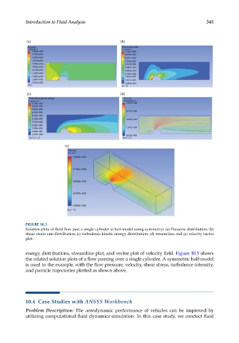
FIGURE 10.5
Solution plots of fluid flow past a single cylinder (a half-model using symmetry). (a) Pressure distribution; (b)
shear strain rate distribution; (c) turbulence kinetic energy distribution; (d) streamline; and (e) velocity vector
plot.

energy distributions, streamline plot, and vector plot of velocity field. Figure 10.5 shows
the related solution plots of a flow passing over a single cylinder. A symmetric half-model
is used in the example, with the flow pressure, velocity, shear stress, turbulence intensity,
and particle trajectories plotted as shown above.

10.4 Case Studies with ANSYS Workbench

Problem Description: The aerodynamic performance of vehicles can be improved by
utilizing computational fluid dynamics simulation. In this case study, we conduct fluid